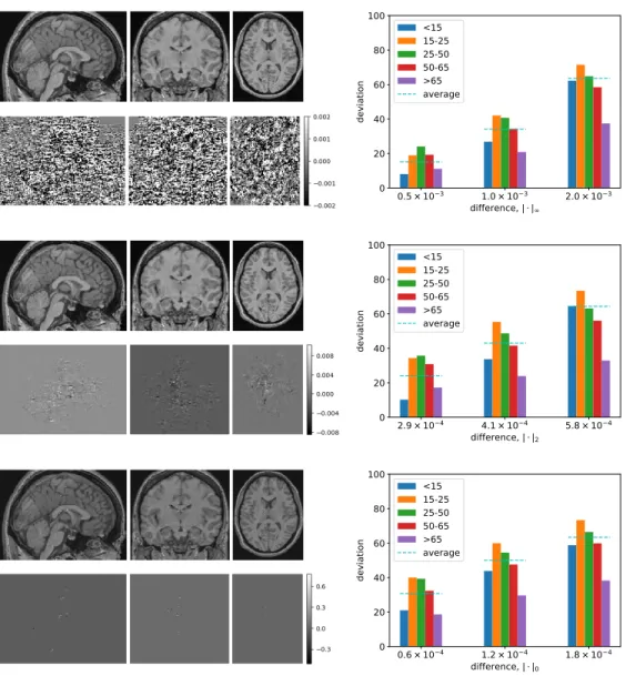
The images in the top row of each of these correspond to the modified 2D slice images of the brain; directly below that is isolated noise that we add (amplified for visibility). In each graph, the x-axis is the limit on the amount of noise injected (where the noise limit is measured by each of our three measurements), while the y-axis is the corresponding impact, measured as deviation from the original prediction.
Motivation
While deep learning has recently become prominent in medical imaging, there is growing concern about its clinical safety given the algorithmic complexity of neural networks. The "black box" nature of the neural network makes it difficult to describe which features are driving the models, thus limiting its application in clinical use.
Research Challenges
Challenge 1: White Matter Lesion Segmentation is Difficult
Additionally, in the computer vision community, many studies have investigated the vulnerability of deep learning models to unexpected perturbations, commonly known as adversarial examples. Furthermore, deep learning outperformed other methods due to its ability to create features directly from the training data without any manual feature engineering.
Challenge 2: Inaccurate Morphological Analysis with Presence of Lesions 4
For many MS lesion segmentation challenges, deep learning-based methods have achieved top rankings with the development of deep learning theory and increased computing power. On the other hand, this means that deep learning-based approaches usually need a large amount of training data to achieve outstanding performance.
Challenge 4: CNN Models Are Vulnerable to Adversarial Attacks
Contributions
Addressing Challenge 1: Improving White Matter Lesion Segmentation 7
In order to alleviate the dependence of the inpainting algorithm on the accurate lesion delineation, I propose a robust multiple sclerosis inpainting algorithm with the edge in front. If the task requires the model to preserve topological structure while discarding all intensity values around the ROI, then the boundary condition will be useful.
Addressing Challenge 3: Cross-Datasets Model Adaptation
Addressing Challenge 4: Adversarial Defense with Anatomical Features 10
Overview
Datasets
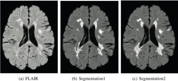
Three experts (1 from CHB, 2 from UNC) segmented the lesion manually, while only the delineations from the CHB expert are provided for the training set. For each subject, it contains 4 to 5 time point MRI scans, resulting in a total of 21 images for the training set.

Lesion Segmentation
Unsupervised Methods
To make better use of assessment from more than one modality, Forbes et al.[47] proposed a method to adaptively calculate the relative weight of each sequence using the EM algorithm. An example is [50], which uses Mean Shift as a segmentation method to generate local regions.
Supervised Methods
Royet al.[97] used a fully convolutional neural network (FLEXCONN) to obtain the segmentation of the 3D input patch. More recently, Aslanite al.[6] proposed a 2D end-to-end deep neural network and its contribution.
Lesion Inpainting
MS Lesion Inpainting
Valverde et al.[113] performs the re-filling slice-by-slice and the lesion voxels are filled by the random values generated from the Gaussian distribution estimated by the white matter intensity of the current slice. Recently, a deep learning inpainting method has been presented by Xiong et al.[120] for multiple sclerosis lesions.
Natural Image Inpainting
In Yang et al.[123] the authors use the context encoder as the content network, while using another texture network to optimize the local texture loss. Iizuka et al.[62] proposed to use the global GAN loss (of the whole image) and the local GAN loss (of the ROI) at the same time.
Robustness in Medical Imaging
Cross-dataset Robustness
Weeda et al.[119] further test the one-shot learning proposed by [114] with an independent data set, and the performance is better than unsupervised methods and is comparable to fully trained supervised methods. Baure et al.[14] propose to train an autoencoder for unsupervised anomaly detection in the target domain, and use this unsupervised model to generate artificial labels for joint training of a supervised model with labeled data from the source domain.
Robustness to Adversarial Attack
Problem Overview
I performed experiments on our in-house dataset and the ISBI 2015 Longitudinal MS Lesion Segmentation Challenge dataset (Challenge). The ablation experiments show that the introduction of 2.5D stacked slices is helpful for the segmentation performance, and the Tiramisu model outperforms U-Net.
Materials and Methods
Datasets and Pre-processing
- In-house Dataset
- ISBI Longitudinal MS Lesion Segmentation Challenge Dataset 29
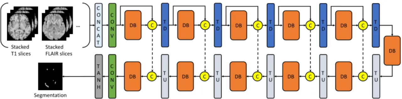
For the internal dataset, T1-w and FLAIR images were co-registered to T1-w space using ANTs [9] and de-skulled using BET [103]. For a multimodal dataset of N modalities (for example, N = 4 for the Challenge dataset containing T1-w, T2-w, FLAIR, and PD images), the input would be the concatenation of N stacked slices from the same location from different modalities.
Network Structure and Loss Functions
The term 2.5D is defined as stacked slices along three orthogonal planes (axial, coronal and sagittal). Within each DB, the input for each layer is the concatenation of all the previous layers.
Experimental Methods
Evaluation Metrics and Compared Methods
The downsampling path consists of a convolutional layer (CONV), 5 dense blocks (DB) and the transition down (TD) blocks. The upsampling path is symmetrical to the downsampling path, but for each block's input, the output of the Transition Up (TU) block and the output of the corresponding downsampling block are concatenated.
Implementation Details
Our networks were trained using the Adam optimizer [68] with an initial learning rate (lr) of 0.0002 and a momentum term of 0.5.
Results
Simulated In-house Dataset
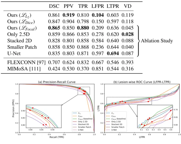
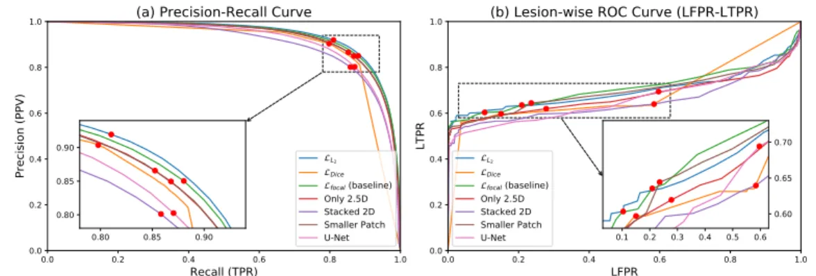
Similarly, when we only use stacked 2D data or use U-Net, the performance is not as good as the baseline. In terms of lesional metrics, the baseline method also showed better performance than the networks in the ablation study.
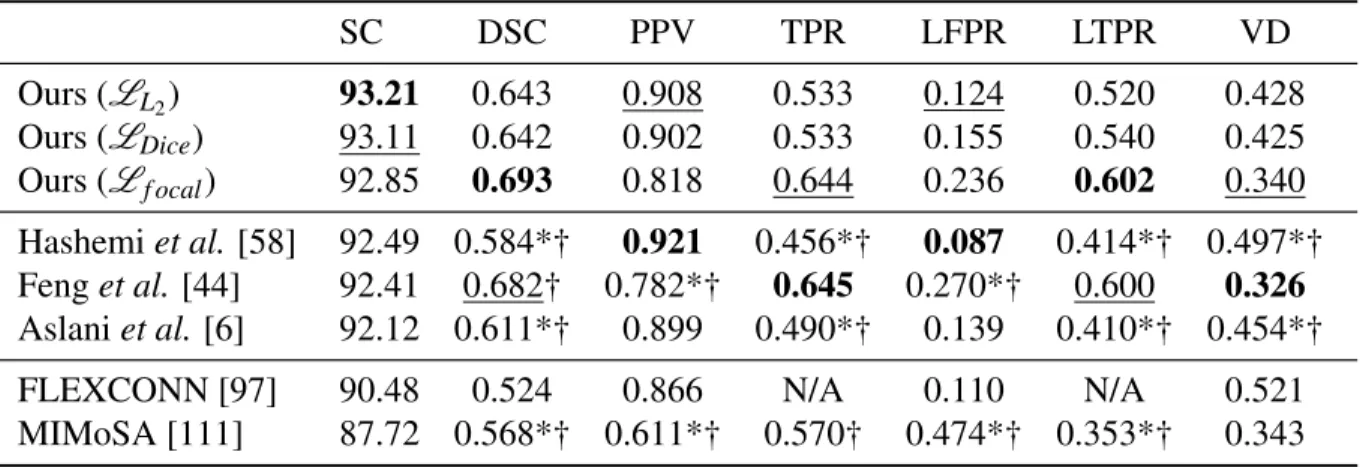
The Longitudinal MS Lesion Segmentation Challenge
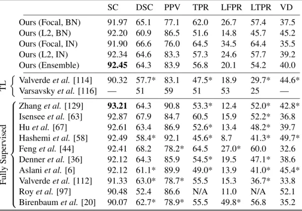
The last two rows are the results obtained with FLEXCONN and MIMoSA based on the same dataset. Similar to our results on the simulated dataset, among the networks, the L2variant has the best overall performance (the highest score).
Conclusion
The focal loss variant achieved the best DSC, the best LTPR, and the second best TPR (recall), indicating that it is highly sensitive to the lesions. I achieved the best overall score with the use of L2 loss and the highest DSC/LTPR with the focal loss.
Problem Overview
Instead of considering the lesion areas as missing, I use the edge information extracted from the input image as a prior guide for inlining. Our method makes no assumptions about the characteristics of the lesions, which makes it suitable for both white matter lesions and gray matter lesions.
Materials and Methods
Datasets and Pre-processing
In this chapter, I refer to the healthy controls as original healthy control (OHC) images and the generated images as simulated lesion images (SL, see Section 3), in contrast to real lesion (RL) images from patients with MS. In the testing phase, I use simulated lesion images (see section 3) for both qualitative and quantitative experiments; I also present quality results from real lesion images.
Edge Detection
By adding some Gaussian noise to B-1 and detecting its edges, we get B-3, which contains some random edges compared to (B-2). I imagine that with these augmentations the network will learn to deal with the edges caused by the lesions.
Network Structure and Loss Functions
To alleviate this discrepancy and teach the model to ignore some edges while preserving others, I use adding input edges during the training phase. The input is the concatenation of the binary lesion mask, masked T1-w, and T1-w edge detection after adding random noise.
Experimental Methods
- Ground truth
- Implementation Details
- Evaluation Metrics
- Compared Methods
Vgt ×100% whereVoandVgt is the volume of a given class in the segmentation of the inpainting output and the ground truth respectively. The F1 score and Jaccard coefficient of similarity (IoU) across all classes are also reported to provide an overall evaluation of the segmentations.
Results
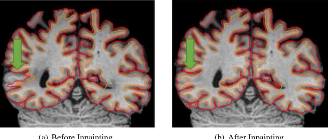
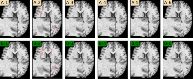
Qualitative Analysis
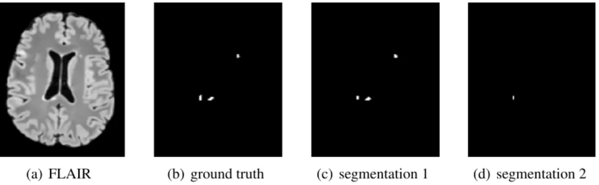
This is due to the merging of the input non-lesion regions and the output lesion regions. We note that the lesion between the lateral ventricles is missing from the lesion segmentation algorithm and is thus not stained by any of the methods.
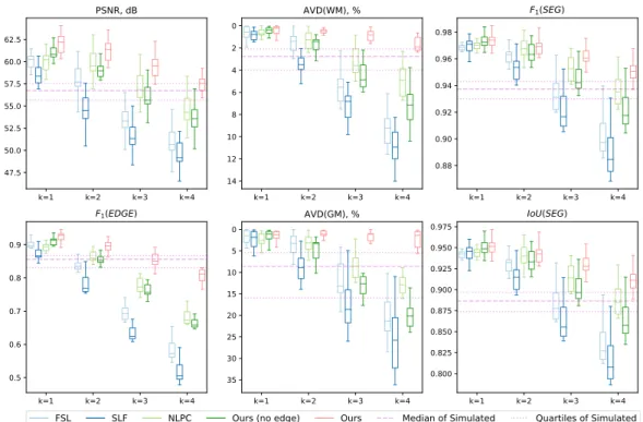
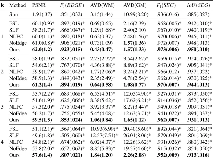
Quantitative Analysis
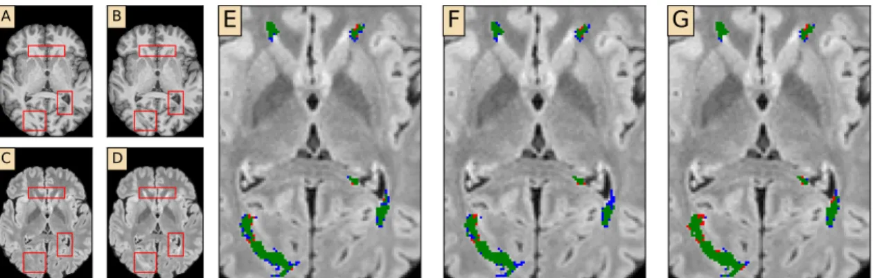
For AVD of WM and GM, our method outperformed all other painting methods and simulated images even when k=4, which is not the case for any of the other methods. As an ablation study, the results of our method without edge advance are also given in Figs.
Conclusion
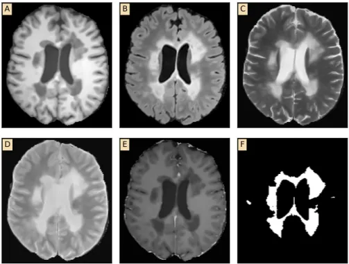
The measurement data is calculated between the processed images and the ground truth lesion-free images. The metrics WM and GM are the percentage deviation of white matter classification and gray matter classification, respectively.
Problem Overview
I propose to help lesion segmentation models to generalize to unseen domains by introducing data additions and mode dropouts (Sec. I also evaluate our models trained on the Longitudinal MS Lesion Segmentation Challenge, which is a domain invisible during training.
Materials and Methods
Datasets
Data Augmentations and Modality Dropout
Network Structure and Loss Functions
Experimental Methods
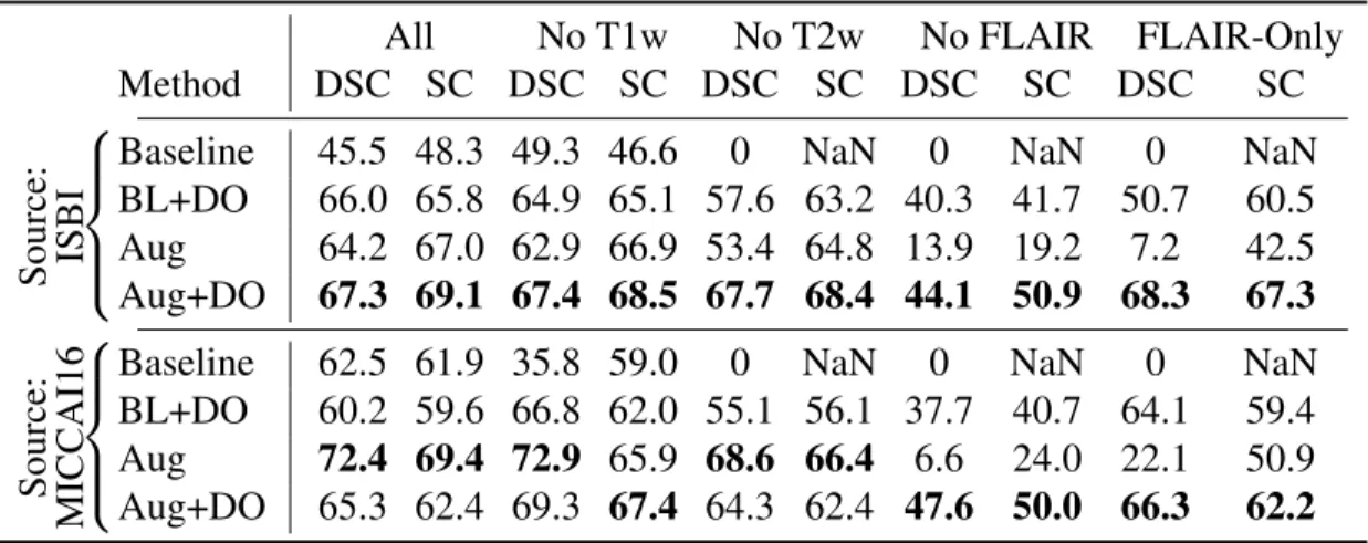
Compared methods. Many state-of-the-art methods, most of which are fully supervised [128], have provided their results on the ISBI challenge dataset. 114] trained networks with two public databases (MIC-CAI08 [105], MICCAI16) and then fine-tuned them with a single subject from the ISBI database.
Results
Domain Generalization without Modalities Missing
However, for models trained with the UMCL dataset, the two methods had similar results. We note that the cross-validation results of supervised models trained on the ISBI database are 77.0% for Dice.
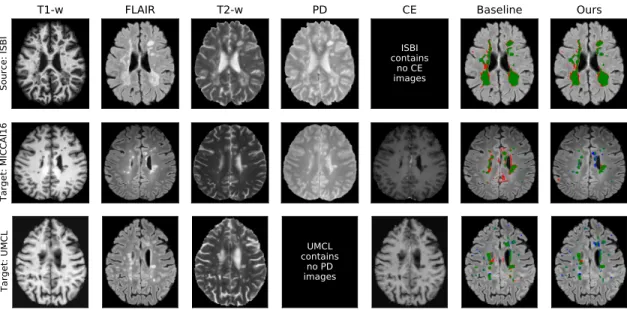
Domain Generalization with Missing Modalities
DSC SC DSC SC DSC SC. with more training images and approaches the 'upper bound' of supervised models. However, models trained with Aug or Aug+DO are much more robust than BL or BL+DO.
Evaluation on the ISBI test set
Among these, the Focal Loss + BN variant is consistent with all the experiments presented in previous sections. Note that using only MICCAI16, a smaller dataset than UMCL, I am able to get a score of 91.98 (using L2+IN, data not presented).
Conclusion
Note that the SC is re-scaled for this challenge, so 90 means human-level performance. ISBI Challenge takeaway: My models outperform existing transfer learning methods and achieve performance comparable to supervised methods.
Problem Overview
In addition, potential harmful consequences of the opacity of deep learning have recently come to the fore in the computer vision community (mainly focusing on image classification tasks), where several studies reveal the vulnerability of deep learning models to unexpected perturbations, commonly known as counterexamples. Our third contribution is to experimentally demonstrate that adversarial exemplars – both image-specific and universal – are indeed extremely effective, significantly reducing the prediction efficiency of deep learning for age prediction.
Experimental Methods
Generating Adversarial Perturbations for a Single Image
- The l ∞ Attack
- The l 2 Attack
- The l 0 attack
If our goal is to minimize rather than maximize life expectancy, the goal becomes minimization rather than maximization. To minimize the predicted age, the only difference is to change the value of one pixel in each iteration to make the prediction smaller instead of larger.
Generating Adversarial Perturbations for a Batch of Images
Results
Conventional Deep Neural Networks are Fragile to Adversarial Pertur-
As we can see from the illustration (pictures in the left column of the figure), we can cause the conventional DNN to predict age as 80 (rather than 19) by any of the three ways of quantifying disorder, with all three brain images looking similar indistinguishable from the original (in Figure 6.1(a)). A more systematic analysis in Figure 6.3 (plots in the right column) shows that age can be boosted by nearly 70 years on average by adding perturbation of magnitude <0.002 (for the normalized image) to any of the three measures.
A Single Adversarial Perturbation Works for Large Batches of Images . 74
The images in the left column show the results of the adversarial perturbations in the image of the 19-year-old subject in Fig. 6.1(a), using each of our three criteria for limiting the size of the perturbations. Consider Figure 6.6, which presents a systematic analysis of the impact of adversarial perturbations on a context-aware model.1 The difference with a conventional DNN is obvious: in each case, the impact of the attack is significantly reduced, often by several factors.
Discussion
However, our results also suggest that a way to address the fragility of deep learning models is to incorporate domain knowledge and more traditional multi-atlas image segmentation techniques. In this dissertation, I mainly focus on improving the automatic quantification of MS lesions using deep learning models.
Summary of Contributions
The techniques developed in this thesis also have the potential to be applied to other medical imaging research. Further, I believe that many deep-learning-based medical image models with multimodal input are able to generalize to unseen domains by combining strong data augmentation and modality dropout.
Future Work
Cortical Lesions Segmentation
Ground truth markers of cortical lesions will be characterized using postmortem 7T MRI and postmortem histopathology, which are considered the “gold standard”. When segmenting 3T images, 7T scans will be used to resolve ambiguity, but invisible lesions in 3T will not be flagged.
Lesion Inpainting Independent of Segmentation
A self-adaptive network for segmentation of multiple sclerosis lesions based on multi-contrast MRI with different image sequences”. OASIS is automated statistical inference for segmentation, with applications to segmentation of multiple sclerosis lesions in MRI”.