We hope that this book will encourage more and more people to use R to do data mining work in their research and applications. This chapter introduces basic data mining concepts and techniques, including a data mining process and popular data mining techniques.
Data Mining
It presents many examples of different data mining functionalities in R and three case studies of real world applications. The assumed audience for this book is postgraduate students, researchers, and data miners interested in using R to conduct their data mining research and projects.
Datasets
The Iris Dataset
To help users determine which R packages to use, the CRAN Task Views6 are a good guide. Another guide to R for data mining is an R data mining reference card (see page ??), which provides a comprehensive indexing of R data mining packages and functions, categorized by their functionalities.
DATASETS 3
The Bodyfat Dataset
This chapter shows how to import foreign data into R and export R objects to other formats. Initially, examples are given to demonstrate how R objects are stored and loaded from .Rdata files.
Save and Load R Data
For more details on data import and export, please refer to R Data Import/Export 1[R Development Core Team, 2010a].
Import from and Export to .CSV Files
Import Data from SAS
Import/Export via ODBC
Read from Databases
Output to and Input from EXCEL Files
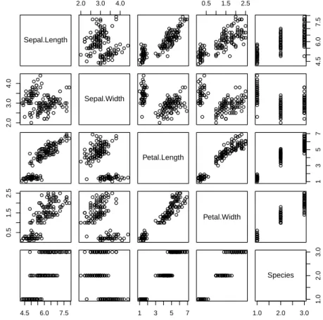
Exploration of multiple variables is then demonstrated, including clustered distribution, clustered boxplots, scatter plots, and pair plots.
Have a Look at Data
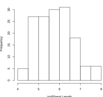
For example, the first 10 values of Sepal.Length can be retrieved using one of the codes below.
EXPLORE INDIVIDUAL VARIABLES 11
Explore Individual Variables
Then we check the variance of Sepal.Lengthwithvar() and also check its distribution with histogram and density using functionshist()anddensity().
EXPLORE INDIVIDUAL VARIABLES 13
EXPLORE MULTIPLE VARIABLES 15
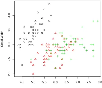
Explore Multiple Variables
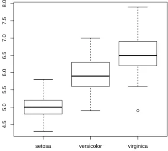
We then use function boxplot() to plot a box plot, also known as a box-and-whisker plot, to show the median, first and third quartiles of a distribution (i.e. the 50%, 25% and 75% points in cumulative distribution), and outliers. The box shows the interquartile range (IQR), which is the range between the 75% and 25% observation.
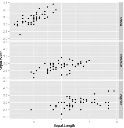
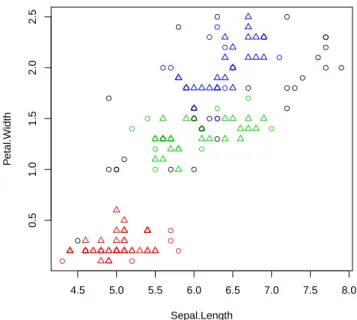
EXPLORE MULTIPLE VARIABLES 17 and symbols (pch) of points are set to Species
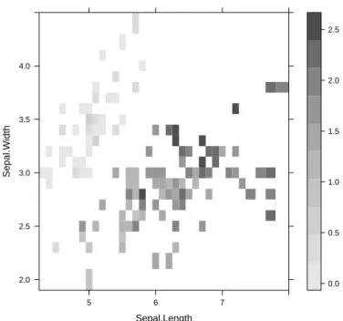
More Explorations
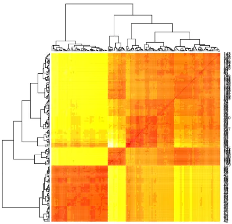
MORE EXPLORATIONS 21 with dist() and then plot it with a heat map
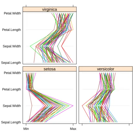
MORE EXPLORATIONS 23 with contourplot() in package lattice
MORE EXPLORATIONS 25 package lattice
SAVE CHARTS INTO FILES 27
Save Charts into Files
It starts with building decision trees with the package party and using the constructed tree for classification, followed by another way to build decision trees with the package rpart.
Decision Trees with Package party
After that, we can take a look at the constructed tree by typing the rules and drawing the tree.
DECISION TREES WITH PACKAGE PARTY 31
Decision Trees with Package rpart
DECISION TREES WITH PACKAGE RPART 33
DECISION TREES WITH PACKAGE RPART 35
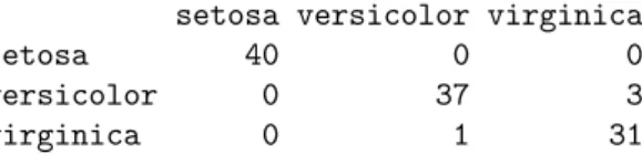
Random Forest
RANDOM FOREST 37 setosa versicolor virginica
RANDOM FOREST 39
First, it shows an example of building a linear regression model to forecast CPI data. Next, the generalized linear model (GLM) is presented, followed by a brief introduction to nonlinear regression.
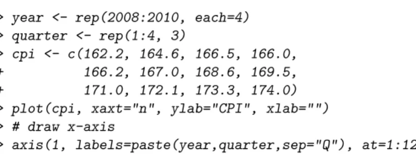
Linear Regression
A collection of some useful R functions for regression analysis is available as a reference card at R Functions for Regression Analysis 1. Next, the lm() function is used to build a linear regression model on the above data using year and quarter as predictors and CPI as the response.
LINEAR REGRESSION 43 With the above linear model, CPI is calculated as
We can also plot the model in a 3D plot, as below, where the scatterplot3d() function creates a 3D scatter plot and plane3d() draws the matching plane.
LINEAR REGRESSION 45
Logistic Regression
GENERALIZED LINEAR REGRESSION 47
Generalized Linear Regression
If family=gaussian("identity") is used in the code above, the model built would be similar to linear regression.
Non-linear Regression
This chapter presents examples of various clustering techniques in R, including k-means clustering, k-medoid clustering, hierarchical clustering, and density-based clustering. The last section describes the idea of density-based clustering and the DBSCAN algorithm and shows how to cluster with DBSCAN and then label new data with the clustering model.
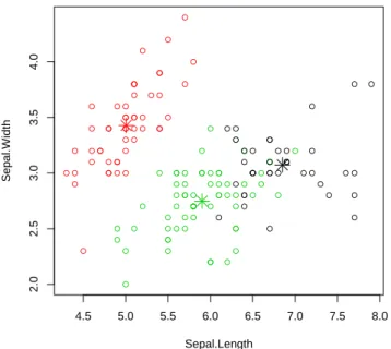
The k-Means Clustering
For readers unfamiliar with clustering, introductions to various clustering techniques can be found in [Zhao et al., 2009a]. We should also be aware that k-means clustering results may vary from run to run, due to random selection of initial cluster centers.
THE K-MEDOIDS CLUSTERING 51
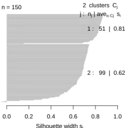
The k-Medoids Clustering
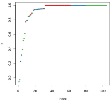
In the example above, pamk() produces two groups: one is "setosa" and the other is a mixture of "versicolor" and "virginica". In the silhouette, largesi (almost 1) indicates that the corresponding observations are very well clustered, smallsi (around 0) means that the observation is between two clusters, and observations with a negative si are likely to be placed in the wrong cluster.
HIERARCHICAL CLUSTERING 53
Hierarchical Clustering
Similar to the k-means clustering above, Figure 6.4 also shows that the setosa cluster can be easily separated from the other two clusters, and that the versicolor and virginica clusters overlap to a small degree. the other.
Density-based Clustering
DENSITY-BASED CLUSTERING 55
DENSITY-BASED CLUSTERING 57 You can use the clustering model to label new data based on the similarity between the new data.
DENSITY-BASED CLUSTERING 57 The clustering model can be used to label new data, based on the similarity between new
An example of outlier detection using LOF (Local Outlier Factor) is then given, followed by examples of outlier detection by clustering.
Univariate Outlier Detection
The aforementioned bias detection can be used to find outliers in multivariate data in a simple ensemble manner.
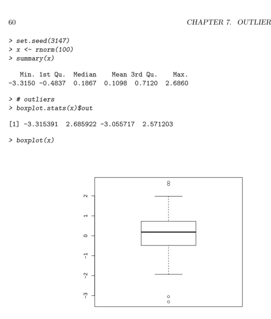
UNIVARIATE OUTLIER DETECTION 61
When there are three or more variables in an application, a final list of outliers can be produced by majority voting of outliers found from individual variables.
Outlier Detection with LOF
OUTLIER DETECTION WITH LOF 63
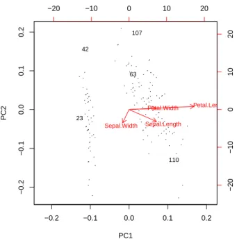
In the code above, prcomp() performs principal component analysis, and biplot() plots the data using the first two principal components. We can also display outliers using a pairs chart, like the one below, where outliers are labeled “+” in red.
OUTLIER DETECTION WITH LOF 65
Outlier Detection by Clustering
OUTLIER DETECTION FROM TIME SERIES 67
Outlier Detection from Time Series
Discussions
DISCUSSIONS 69 Some other R packages for outlier detection are
The second section shows an example on the decomposition of time series into trend, seasonal and random components. The fourth section introduces Dynamic Time Warping (DTW) and hierarchical clustering of time series data with Euclidean distance and DTW distance.
Time Series Data in R
The fifth part shows three examples of time series classification: one with original data, one with DWT (discrete wavelet transform) transformed data, and one with k-NN classification.
Time Series Decomposition
TIME SERIES DECOMPOSITION 73
The second is trend of the data, the third shows seasonal factors, and the last graph is the remaining components after removing trend and seasonal factors. Some other functions for time series decomposition arestl()in packagestats [R Development Core Team, 2012], decomp()in packagetimsac [The Institute of Statistical Mathematics, 2012], entsr()in packageeast.
Time Series Forecasting
TIME SERIES CLUSTERING 75
Time Series Clustering
Dynamic Time Warping
Synthetic Control Chart Time Series Data
TIME SERIES CLUSTERING 77
Hierarchical Clustering with Euclidean Distance
CLUSTERING OF TIME SERIES 79The clustering result in Figure 8.7 shows that the increasing trend (class 3) and upward shift.
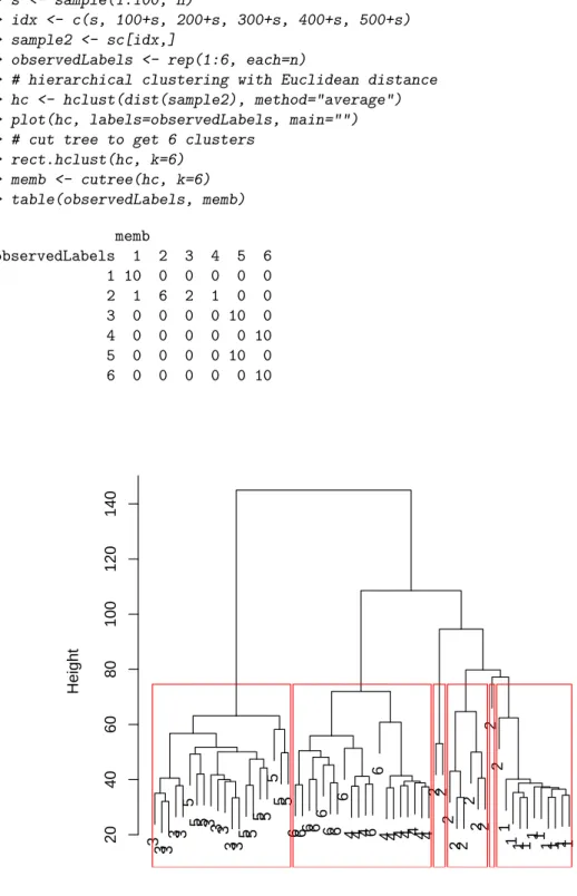
TIME SERIES CLUSTERING 79 The clustering result in Figure 8.7 shows that, increasing trend (class 3) and upward shift
Hierarchical Clustering with DTW Distance
Comparing Figure 8.8 with Figure 8.7, we can see that the DTW distance is better than the Euclidean distance for measuring the similarity between time series.
TIME SERIES CLASSIFICATION 81
Time Series Classification
Classification with Original Data
Classification with Extracted Features
TIME SERIES CLASSIFICATION 83 and V contains scaling coefficients. The original time series can be reconstructed via an inverse
For the 20 nearest neighbors of the new time series, three are from class 4, and 17 are from class 6. By majority voting, i.e. by taking the more frequent label for the winner, the label of the new time series is determined up to class 6.
Discussions
It finds the nearest neighbors of the new instance and then marks it by majority vote. However, the time complexity of the naive nearest neighbor search method is O(n2), where is the size of the data.
Further Readings
It starts with basic concepts of association rules, then demonstrates association rule mining with R. It then presents examples of pruning redundant rules and interpreting and visualizing association rules.
Basics of Association Rules
The Titanic Dataset
Association Rule Mining
In the above resultrules.all we can also see that the left side (lhs) of the first rule is empty. When other settings are unchanged, with a lower minimum support, more rules will be produced and the associations between item sets shown in the rules will be more random.
Removing Redundancy
INTERPRETING RULES 91
Interpreting Rules
Visualizing Association Rules
VISUALIZING ASSOCIATION RULES 93
VISUALIZING ASSOCIATION RULES 95
Discussions and Further Readings
Finally, words and tweets are clustered to find clusters of words as well as clusters of tweets. In this chapter, "tweet" and "document" will be used interchangeably, as will "word" and "expression".
Retrieving Text from Twitter
Therefore, this book uses the following code to print the five tweets by wrapping the text to fit the width of the paper. 13]] Postdoc on optimizing a cloud for data mining primitives, INRIA, France http://t.co/cA28STPO.
Transforming Text
11]] Slides on massive data, shared and distributed memory, and concurrent programming: bigmemory and foreach http://t.co/a6bQzxj5. 14]] Chief Scientist - Data Intensive Analytics, Pacific Northwest National Laboratory (PNNL), USA http://t.co/0Gdzq1Nt.
Stemming Words
Below we focus on point 3, where the word "mining" first derives from "mine" and then completes into "miner", instead of "mining", although there are many instances of "mining" in the tweet, compared to only two. cases of "miners". Instead, we chose a simple way to overcome it by replacing "miners" with "mining", since the latter has many more occurrences than the former in the corpus.
Building a Term-Document Matrix
As we can see from the above results, there is something unexpected in the above formation and completion. In the above editions, point 1 is caused by the missing space after the comma.
Frequent Terms and Associations
The barplot in Figure 10.1 clearly shows that the three most frequent words are "r", "data" and. Below we try to find terms related to "r" (or "mining") with a correlation of no less than 0.25, and the words are sorted according to their correlation with "r" (or "mining").
Word Cloud
The above word cloud again clearly shows that “r”, “data” and “mining” are the top three words, confirming that the @RDataMining tweets present information about R and data mining. Another set of frequent words, "research," "postdoc," and "positions," came from tweets about postdoctoral and research job vacancies.
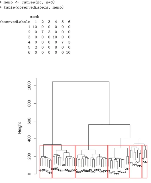
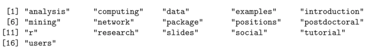
Clustering Words
Some other important words are "analysis", "examples", "slides", "tutorial" and "package", which shows that it focuses on documents and examples on analysis and R packages. There are also some tweets on the topic of social network analysis, as indicated by words "network" and "social" in the cloud.
CLUSTERING TWEETS 105
Clustering Tweets
Clustering Tweets with the k-means Algorithm
Note that a fixed random seed is set withset.seed() before running kmeans(), so that the clustering result can be reproduced. It's for ease of writing books and it's unnecessary for readers to put a random seed in their code.
CLUSTERING TWEETS 107 + # print(rdmTweets[which(kmeansResult$cluster==i)])
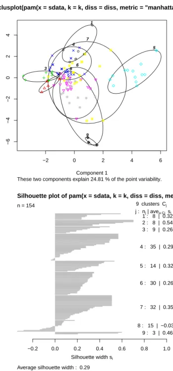
Clustering Tweets with the k-medoids Algorithm
In Figure 10.4, the first plot is a 2D clusterplot of the k clusters, and the second shows their silhouettes.
Packages, Further Readings and Discussions
This chapter presents examples of social network analysis with R, specifically with packageigraph [Csardi and Nepusz, 2006]. In this chapter, we first build a network of terms based on their co-occurrence in the same tweets, and then we build a network of tweets based on the terms they share.
Network of Terms
Putting it in a general social networking scenario, terms can be taken as people and tweets as groups on LinkedIn1, and the term-document matrix can then be taken as people's group membership. In the code above, %*% is an operator for the product of two matrices, andt() transposes a matrix.
NETWORK OF TERMS 113
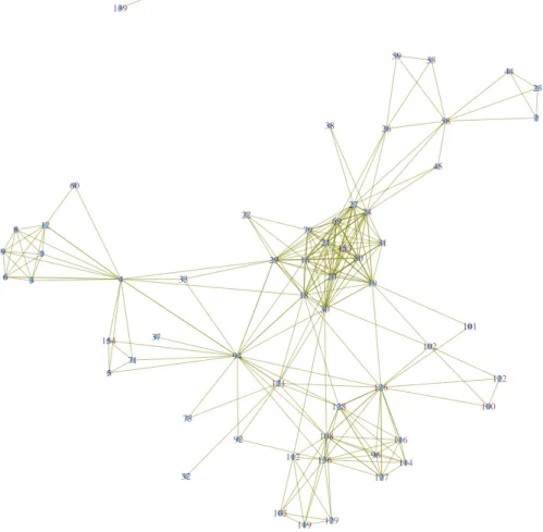
Network of Tweets
NETWORK OF TWEETS 115
NETWORK OF TWEETS 117
6] Parallel Computing with R Using Snow and Snowfall http://t.co/nxp8EZpv [9] R with High Performance Computing: Parallel Processing and Large Memory http://t.co/XZ3ZZBRF. 8] Slides on parallel computing in R http://t.co/AdDVxbOY [3] Easier parallel computing in R with snowfall and sfCluster.
Two-Mode Network
TWO-MODE NETWORK 121 An alternative way is using function neighborhood() as below
From Figure 11.8, we can clearly see groups of tweets and their keywords, such as time series, social network analysis, parallel computing, and postdoc and research positions, which are similar to the result at the end of Section 11.2.
Discussions and Further Readings
DISCUSSION AND FURTHER READING 123 are also packages designed for topic modeling, such as the lda package [Chang, 2011] and topic models.
DISCUSSIONS AND FURTHER READINGS 123 are also packages designed for topic modeling, such as packages lda [Chang, 2011] and topicmodels
Summary: This chapter presents a case study on the analysis and forecasting of House Price Indices (HPI). Summary: This chapter presents a case study on the use of decision trees to predict customer response and optimize profit.
R Reference Cards
Using R for Data Analysis and Graphics - Introduction, Examples and Comments http://www.cran.r-project.org/doc/contrib/usingR.pdf. Many contributed R docs, including non-English http://cran.r-project.org/other-docs.html.
Data Mining
Resources to help you learn and use R at UCLA http://www.ats.ucla.edu/stat/r/.
DATA MINING WITH R 133
Data Mining with R
Classification/Prediction with R
Time Series Analysis with R
Association Rule Mining with R
Spatial Data Analysis with R
Text Mining with R
Social Network Analysis with R
DATA CLEANSING AND TRANSFORMATION WITH R 135
Data Cleansing and Transformation with R
Big Data and Parallel Computing with R
An improved representation of time series enabling fast and accurate classification, clustering and relevance feedback. Data mining with R, learning with case studies. extremevalues, an R package for outlier detection in univariate data.