In this thesis, we note the error of the approximation algorithms [41] for sweep coverage for a set of points. The objective of the sweep coverage problem is to find a minimum number of mobile sensors to guarantee sweep coverage for a given set of POIs.
Scope of the Thesis
- Sweep coverage for a set of points
- Sweep coverage with heterogeneity
- Solving energy issues for sweep coverage
- Area sweep coverage
- Barrier sweep coverage
- Distributed sweep coverage
We introduce an energy-constrained sweep covering problem for single curve and propose a 133 approximation algorithm. For multiple curves in a plane, we propose a 5-approximation algorithm for barrier sweep covering problem and a 2-approximation algorithm for a special case of the problem.
Static coverage
Point coverage
69] proposed a centralized greedy heuristic to construct disjoint sensor arrays for energy-efficient target monitoring. The goal of the problem is to find the maximum number of strings among a set of sensors.
Area coverage
In paper [16], the authors considered a geometric version of the point coverage problem called unit disc cover problem. If some unclipped sensors are located within the hexagon of a broken sensor, then the clipped sensor pushes these unclipped sensors to the lower density area of the plane.
Barrier coverage
The authors addressed the problem of covering a set of line segments by a minimum number of sensors with uniform observation range of the sensors. Different deterministic algorithms are proposed to solve the above problems for a set of line segments with different properties.
Sweep coverage
Contribution
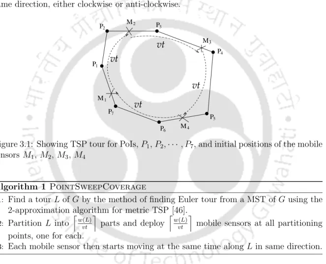
In the optimal solution, each mobile sensor should move along the optimal TSP tour between the PoIs. Each point on L can be visited by at least one mobile sensor in each time period t.
Sweep Coverage on a Weighted Graph
Analysis
Let opt0 be the smallest number of paths with weight ≤vt which span U onG and M in path be the sum of the weights of all such paths. If Ci is a component with more than one vertex, then the number of partitions on Ci is l2w(Ci).
Sweep Coverage in Presence of Obstacles
The time complexity of Algorithm 2 is O((n+k)3), where n is the number of PoIs and k is the total number of vertices of the polygonal obstacles. The total number of vertices of the visibility graph Gv is (n +k), since Gv is constructed with all PoIs and vertices of the polygonal obstacles.
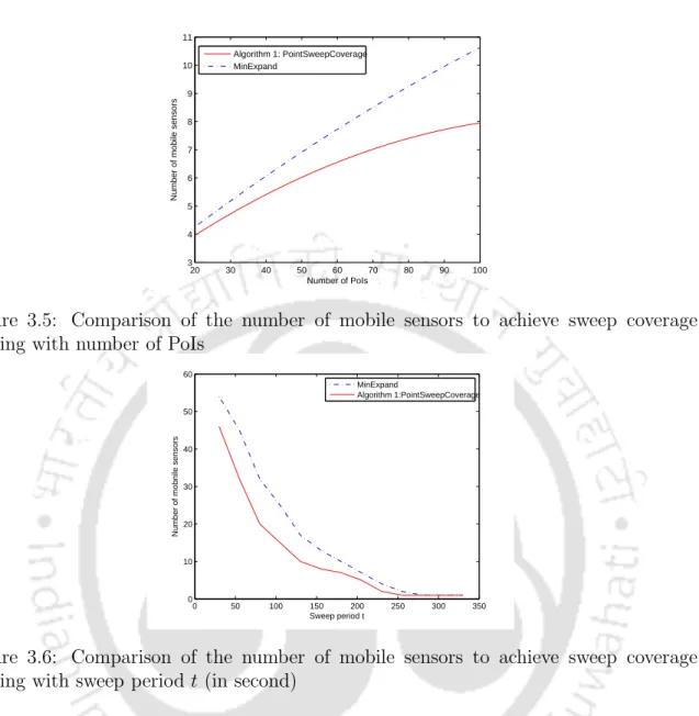
Simulation
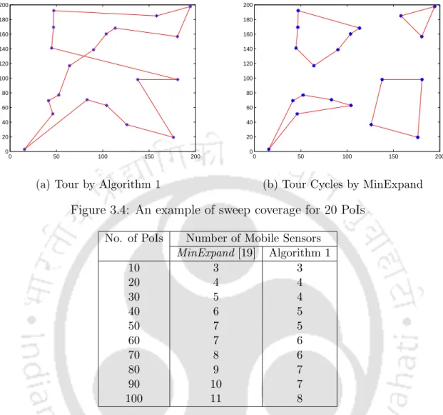
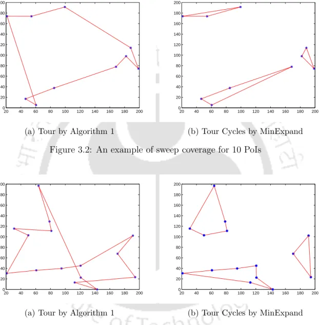
An example of mobile sensor tours for 10 PoIs is shown in Fig. 3.2a shows the output of the tour from Algorithm 1, where the length of the tour is 468.9 meters and the required number of mobile sensors is 2. The average mobile sensor number is calculated for 100 several runs of the algorithms with a sweep period of 200 seconds.
Conclusion
Contribution
We propose an approximation algorithm to solve the sweep coverage problem for a weighted graph when the vertices of the graph have different sweep periods. If the speeds of the mobile sensors are different, we prove that it is impossible to design a constant factor approximation algorithm to solve the sweep coverage problem unless P = NP.
Sweep Coverage with Different Sweep Periods and Processing Times
Proposed algorithm
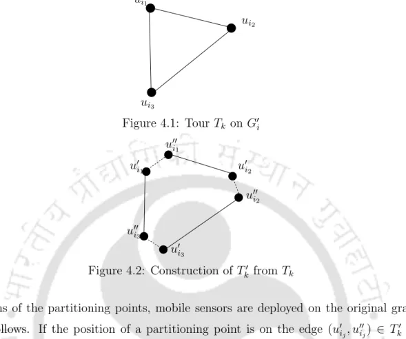
First phase finds number of mobile sensors and second phase calculates movement strategy of the mobile sensors. Now we explain how to deploy the mobile sensors to ensure sweep coverage for all the vertices of G. After deployment, all mobile sensors move around the tour Tk0 in the same direction and the movement of the mobile sensors is reflected in the original graphGas explained below. .
Analysis
Then it moves to the next vertex in the trip along the shortest path of the two vertices with uniform speed v. Then OU Ti ≤ 6OP Ti, since the length of the partition in OP Ti is at most twice the length of the partition in OU Ti and the Algorithm 2 is a 3-approximation algorithm. Although it seems that the time complexity of the algorithm for problem 2 is pseudopolynomial, but according to the decomposition strategy of the vertices of the graph, there can be at most n non-empty disjoint vertex sets.
Inapproximability of Sweep Coverage with Mobile Sensors having Differ-
We consider the case of (G1, L) metric TSP, where G1 = (U1, E1, w1) is a complete weighted graph with n (> k) nodes and the edge weights of G1 are integers and satisfy the triangle inequality. We consider an example of a mobile sensor coverage problem with different speeds as follows: we take G2 as an input graph, a sweep period t = 1, and a set of n2 mobile sensors, among which the speed of one mobile sensor Land is the speed of the rest. Therefore, at least one point from each set {u1i, u2i,· · · , uni} for differentials is visited by a mobile sensor with a travel speed and weight of at most L.
Conclusion
Contribution
We propose a variant of the sweep coverage problem, called the energy-efficient sweep coverage problem or the ESweep coverage problem. For a special case of the above problem, a two-approximation algorithm is proposed, which is the best possible approximation factor. We introduce another variant of the sweep coverage, called the energy-constrained sweep coverage problem or the ERSweep coverage problem, and propose a (5+α2) approximation algorithm to solve this NP-hard problem.
Energy Efficient Sweep Coverage Problem
Algorithm and Analysis
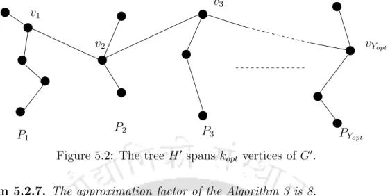
The output of the algorithm is the number of mobile and static sensors with deployment locations for static sensors and motion plan for mobile sensors. An example of the movement paths of the mobile sensors in the optimal solution is shown in fig. According to step 6 of Algorithm 3, the total number of mobile sensors needed is Ykopt, which is.
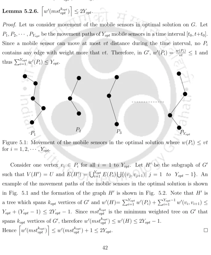
A special case of ESweep coverage problem
LetXopt and Yopt are the number of static and mobile sensors in the optimal solution. Let mobile Yopt sensors visit kopt vertices of G and the remaining n-kopt vertices are covered by Xopt = n-kopt static sensors.
Energy Restricted Sweep Coverage Problem
Algorithm and Analysis
The Algorithm 5 (ERSweepCoverage) is proposed to solve the ERSweep coverage problem that returns the number of mobile sensors needed to guarantee t-sweep coverage of the given set of POIs by maintaining the energy constraint of the mobile sensors. Minimum over the number of partitions of all iterations is chosen as the output of the Algorithm 5. Since Fopt is the minimum spanning forest with opt number of components, opt·vt≥w1(Fopt), that is, opt≥ w1(Fvtopt ).
Conclusion
Contribution
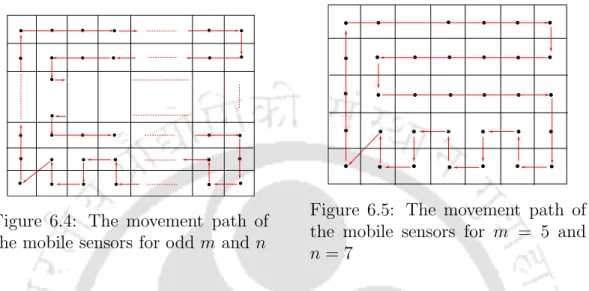
The approximation factor of the proposed algorithm is a function of the area, the perimeter of the area and the detection range of the mobile sensors for an arbitrary bounded area.
Area Sweep Coverage Problem
Solution of Area Sweep Coverage
Analysis
The recovery area 2rvt is covered due to the movement of the mobile sensor along the IF line, which is shown by the white area in the same figure. According to Algorithm 2, the total tour length of the mobile sensors is less than or equal to twice the length of the MST of G. The time complexity of Algorithm 6 is O(m2logm), where m= 2ra22, a is the side of the square region, and r is the sensing radius of the mobile sensors.
Improved Solution for Rectangular Region
After finding the motion cycles in both of the above examples, divide the cycles by L. The approximation factor of the area coverage algorithm for a mesh graph with an even number of vertices is. 2r×mn, the total number of mobile sensors required to cover R isdmn×vt√2re.
Solution for Arbitrary Bounded Region
Each mobile sensor starts moving simultaneously along L in the same direction to cover R. The number of grid points in A is ≤ Area(2r2A) + √P2r, so the number of nodes required to cover P is .
Simulation
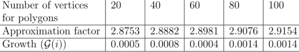
To observe the growth of the approximation factor, we define it as: G(i) =|AF(i)−AF(i−1)|, where AF(i) is the value of the approximation factor for an area being bounded by a simple polygon with i vertices, i.e. AF(i) = 2√. The reason why the approximation factor increases in our simulation is that we increase the number of vertices of the polygon by generating more vertices within a fixed square area of size 1000 x 1000 meters. The nature of the approximation factor is also investigated with respect to the detection radius of the sensors.
Conclusion
Contribution
An energy-constrained barrier coverage problem is defined and a 133 approximation algorithm is proposed to solve it for a finite curve. The barrier coverage problem for multiple finite curves (BSCMC) is also proposed and proven that the problem is NP-hard and cannot be approximated within a factor of 2 unless P=NP. We formulate a data collection problem, which uses a set of data mules to collect data and prove that the problem is NP-hard.
Problem Definitions
To continue sweeping coverage for a long time, each mobile sensor must visit an energy source to recharge or replace its battery. Let Γ be the maximum travel time for a mobile sensor that starts with fully powered battery and maintains uniform speed v until battery power goes down. Let e be an energy source in the aircraft and each mobile sensor can recharge or replace its battery by visiting e.
Barrier Sweep Coverage for a finite Curve
Optimal solution for a finite curve
For given t,Γ>0, find the minimum number of mobile sensors such that C covers the t-barrier and visits each mobile sensor e once in every Γ time period.
Energy restricted barrier sweep coverage
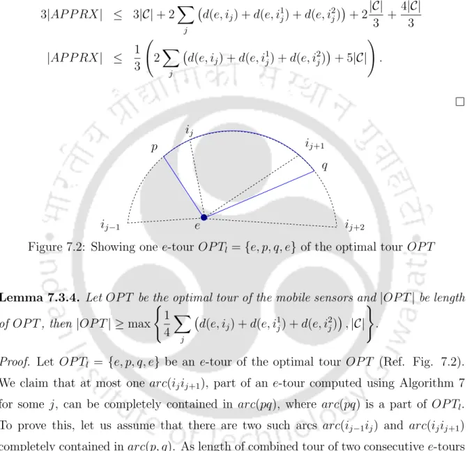
Note that by the construction of e-tours, the combined tour length of any two consecutive e-tours is always greater than vΓ. Divide the AP P RX into equal parts of length and place a removable sensor at each of the split points. Let OP T be the optimal mobile sensor tour and |OP T| be the length of OP T, then |OP T| ≥max.
Barrier Sweep Coverage for Multiple finite Curves
Solution for BSCMC
Let choose the number of mobile sensors required for the optimal solution of BSCMC. Let opt0 be the minimum number of mobile sensors that can guarantee t-sweep coverage of all the vertices of G. Let us consider the movement paths of opt0 number of mobile sensors to sweep the vertices of G in any time interval [t0, t +t0].
Data Gathering by Data Mules
Analysis
Each mobile sensor is visited by a data mule at least once in each t period according to Algorithm 9. Now we consider the case where the mobile sensor moves clockwise from p after time t0. Therefore, regardless of the nature of the movement, a mobile sensor is visited by a data mule at least once in every t time period.
Simulation Results
Conclusion
Contribution
Approximation for a Special Case of Distributed Sweep Coverage
System Model and Algorithm
The mobile sensors start moving along the edges of the Euler tour at the same time after they are all placed. The total number of messages required to find the number of mobile sensors and their initial positions depends on the distributed construction of the MST and finding the Euler tour by doubling each edge of the MST. Perform the remaining steps of Algorithm 10 for each of the components to find the number of mobile sensors and their initial positions.
Conclusion
J2] Barun Gorain og Partha Sarathi Mandal, "Approximation Algorithms for Sweep Coverage in Wireless Sensor Networks", Journal of Parallel and Distributed Computing (Elsevier), Vol. J3 ] Barun Gorain og Partha Sarathi Mandal, "Approximation Algorithms for Barrier Sweep Coverage in Wireless Sensor Networks", Journal of Parallel and Distributed Computing (Elsevier) (indsendt). J4 ] Barun Gorain og Partha Sarathi Mandal, "Solving Energy Issues for Sweep Coverage in Wireless Sensor Networks", Discrete Applied Mathematics (Elsevier), (Sendt).