Existence and extent of impact of individual stock derivatives on spot market volatility in India
Abhilash S. Nair
Indian Institute of Management, Kozhikode 673 570, Kerala, India E-mail: [email protected]; [email protected]
This article first examines the existence of a change in the structure of conditional volatility of stock returns around the time when trading in individual stock derivatives is introduced. Thereafter, it analyses the extent of the structural change between the pre- and post-derivatives regimes, after allowing for asymmetric response to ‘good’ and ‘bad’ news, following the Generalized Autoregressive Conditional Heteroscedastic (GARCH) family of models. Since the exact point of regime change is known for each stock analysed, the article specifies alternative switching asymmetric GARCH (Exponential GARCH (EGARCH), Periodic GARCH (PGARCH) and Glosten–Jagannathan–Runkle GARCH (GJR GARCH)) models for each stock. The final choice of model is made on the basis of the news impact curve. The main finding of this study is that although derivatives seem to enhance the quantity of information transmitted to the spot market, the quality of such information is doubtful, resulting in delayed incorporation of such information into price.
This, the article argues, may be because trading volumes in the Indian derivatives market are dominated by retail investors who lack access to information relevant for trading in the short run. The article then builds a case for introducing longer term derivative instruments for more mean- ingful retail participation.
I. Introduction
The introduction of derivative trading in an asset is expected to attract market players who tend to increase the spot market information efficiency.
These market players can be of three types: (i) hedgers, (ii) arbitrageurs and (iii) speculators.
Further, speculators can be either (completely) informed or partially informed. Since the investment required to buy the derivative instrument is much lesser than buying the underlying asset, hedgers may find derivatives to be a cheaper mode of hedging their spot market exposure. Speculators find the
derivatives market attractive because they could trade in more units of underlying asset for the same investment. Arbitrageurs thrive on mispricing. They remove mispricing in both, the spot and the derivative market, thus linking the asset price in the two markets and in the process making risk- free gains.
Hedgers, arbitrageurs and informed speculators transmit new information into the spot market by taking trading positions in the derivatives market.
Since the asset under discussion is the stock of a company, it is well established in prior research that its return volatility changes with time (Mandelbrot, 1963; Fama, 1965) and is conditional on ‘old’ and
Applied Financial EconomicsISSN 0960–3107 print/ISSN 1466–4305 onlineß2011 Taylor & Francis 1 http://www.informaworld.com
DOI: 10.1080/09603107.2010.534061
‘new’ information. In theory, introduction of deriv- atives trading is expected to change the structure of conditional volatility by reducing the impact of ‘old’
information and increasing the rate at which ‘new’
information is incorporated. Derivatives thus result in greater information efficiency and lower condi- tional volatility in the spot market. However, in the presence of the partially informed speculators, the gains from trading in derivatives would diminish, because trades by the less informed speculators produce noise. Such noise, if transmitted to the spot market does not result in increased information efficiency and reduced conditional volatility.
In India, ‘securities’-based derivative trading started in June 2000, first on index and then on individual stocks. As in other markets, the idea in India was that derivatives would increase the infor- mation efficiency in the spot market and thus reduce conditional volatility. However, this idea may not hold in the presence of partially informed traders.
Hence, after a decade of introduction of trading in individual stock derivatives, it is important to exam- ine its impact on the conditional stock return volatility in the spot market. The aim of this article is to test the existence and extent of the change in structure of conditional volatility of the stock as derivatives are introduced.
This article contributes to the existing empirical literature in a number of ways. First, it illustrates the application of wavelet variance analysis, a more robust approach, to test the existence of change in structure of conditional volatility (Fernandez, 2006).
Second, several prior papers assume the response of conditional volatility to ‘good’ and ‘bad’ news as symmetric. In the case of stock returns, it is well established that its return volatility would respond more to ‘bad’ news as compared to ‘good’ news (Black, 1976; Christie, 1982; Pindyk, 1984; French et al., 1987). To account for this finding, this article specifies appropriate asymmetric Generalized Autoregressive Conditional Heteroscedastic (GARCH) models, for each stock in the sample.
The final choice of model is based on the response of conditional volatility to ‘new’ information as cap- tured by the News Impact Curve (NIC). Third, most prior papers examine the change in structure of conditional volatility by comparing the GARCH coefficients estimated in the pre- and post-derivatives regimes; they do so by making strong distributional assumptions about asset returns in the two regimes. To analyse the structural change in a more general setting and given that the exact point of regime change is known in the case of each stock, this article adopts a Switching Asymmetric GARCH (SAGARCH) specification to model conditional volatility.
The SAGARCH specifications incorporate the inter- action of slope and intercept dummies with the respective parameters of the conditional variance equation. The dummy takes a value zero pre- introduction and one post-introduction of derivatives trading, thus capturing the change in each parameter, across the two regimes. Finally, to the best of my knowledge, this is the most comprehensive (101 stocks) examination to date of the impact of trading in stock derivatives on the conditional volatility of the underlying stock in the Indian context.
The study finds that after trading in derivatives commenced, the information flow to spot market rose for most stocks included in the article. As a result, there seems to be a reduction in the impact of ‘old’
information on conditional volatility. However, this reduction is not due to an increase in the rate at which
‘new’ information is being impounded into spot prices. This may be because most of the volumes in the Indian derivatives market originate from retail investors who lack access to information relevant for trading in the short run. Thus, although there seems to be an increase in ‘new’ information emanating from derivatives market, the reliability of this infor- mation is in question resulting in delayed incorpora- tion of this news in spot asset price. From a policy perspective, it may be argued that introduction of longer term derivative instruments (for periods more than 3 months) would attract more meaningful retail participation, thus reducing the proportion of noise traders in the derivatives market. This policy recom- mendation is in conformity with the views expressed in the report of the derivative market review com- mittee, set up by Securities Exchange Board of India (2008), that ‘longer expiration dates offer the oppor- tunity for longer-term investors to take a view on the price changes without combinations of shorter-term options contract’.
The article is organized as follows: Section II reviews relevant literature and presents gaps in research. Section III elaborates the empirical design of the article. Section IV describes the data and discusses the results and Section V concludes this article.
II. Review of Literature
Ever since the introduction of derivative contracts on financial assets in the early 1980s, there have been a number of studies that examine its impact on the spot market. However, most of these studies have analysed the introduction of index futures (Antoniou and Holmes, 1995; Antoniou et al., 1998; Butterworth,
2000; Gulen and Mayhew, 2000; Bologna and Cavallo, 2002; Bandivadekar and Ghosh, 2003;
Shenbagaraman, 2003). Several papers, which study the impact of individual stock derivative trading on the return volatility of the underlying stock either consider a small sample (Nath, 2003; Vipul, 2006) or are limited to examining the introduction of individ- ual stock futures (Dennis and Sim, 1999).
To highlight the contribution of this article, I classify the existing literature into three categories based on the limitations in these papers that are addressed by my article. First, the introduction of trading in individual stock derivative instruments is expected to change the structure of conditional return volatility. However, before one attributes the struc- tural change to introduction of derivatives trading, it is necessary to check for the existence of such a change (in structure of conditional volatility) around the time when derivatives trading is introduced. Prior studies often do not conduct this test (Antoniouet al., 1998; Dennis and Sim, 1999; Butterworth, 2000;
Gulen and Mayhew, 2000; Bologna and Cavallo, 2002; Bandivadekar and Ghosh, 2003; Nath, 2003;
Shenbagaraman, 2003; Vipul, 2006). Even the few studies that test the existence of structural change in conditional volatility around the time when deriva- tives trading is introduced, do so by including an intercept dummy in the specification of conditional variance. If the dummy significantly explains condi- tional volatility, then it is concluded that there is a change in the structure (e.g. Antoniou and Holmes, 1995). However, two difficulties arise in this line of reasoning: (a) if the dummy is significant, it only means that the conditional volatility has changed and does not necessarily mean that there is a change in its structure, (b) if the dummy is insignificant, then it does not necessarily mean that there is no change in structure of conditional volatility. The structure may have changed in such a way that the level of conditional volatility would remain the same. Two alternative approaches to detect a possible structural change, after allowing for multiple breaks in struc- ture, are the wavelet variance analysis approach and the Cumulative Sum of Squares (CUSUM) approach (Inclan and Tiao, 1994; Aggarwal et al., 1999).
However, Fernandez (2006) finds that the wavelet variance analysis gives superior results as compared to CUSUM estimates. Hence, in this study, a wavelet variance-based approach is adopted to confirm the existence of a change in structure of conditional stock return volatility around the time when derivatives trading is introduced in the said stock.
Second, the existence of asymmetric response of volatility to ‘good’ and ‘bad’ information has been extensively documented in the case of stock returns.
Two reasons put forth for the existence of such a phenomenon are: (i) Leverage Effect (Black, 1976;
Christie, 1982): According to this explanation, a negative return shock leads to a fall in prices and therefore a rise in leverage. Consequently, as ‘bad’
news is incorporated, the perceived riskiness of the stock increases, thus resulting in a further fall in prices and a rise in stock return volatility, (ii) Volatility Feedback (Pindyk, 1984; French et al., 1987; Campbell and Hentschel, 1992): According to this explanation, an expected increase in future volatility leads to higher expected return (as compen- sation to bear this risk) and thereby lowering the stock price. Consequently, one witnesses higher price volatility in response to ‘bad’ news as compared to
‘good’ news. The two explanations differ in their causal linkages. While leverage effect hypothesizes that current negative return shock causes higher future price volatility, volatility feedback effect hypothesizes that anticipated higher future volatility leads to current negative return shock. At the firm level, it is empirically well established that asymmetric response of volatility is primarily due to volatility feedback hypothesis (Bekaert and Wu, 2000).
Volatility feedback or time varying expected return occurs because not all investors react in a rational manner (Antoniou et al., 1998). Such behaviour is typical of market players (investors) who have lower access to information (noise traders). These investors react more strongly to ‘bad’ news than to ‘good’
news. If noise traders are the cause of asymmetry in the market, then introduction of derivatives market may attract the noise traders from the spot market.
Hence, before specifying the structure of condi- tional volatility, one must check whether the response of return volatility to ‘good’ and ‘bad’ news is symmetric. Especially, in the case of individual stocks, since unlike indexes, individual stocks are not diversified. As a result, the change in expected return, caused by the leverage effect or the volatility feedback effect, would be more pronounced in the case of individual stocks as compared to indexes.
To my knowledge, most papers studying the impact of derivatives on spot market return volatility do not test for asymmetric response (Antoniou and Holmes, 1995; Antoniou et al., 1998; Bologna and Cavallo, 2002; Bandivadekar and Ghosh, 2003; Nath, 2003; Shenbagaraman, 2003; Pok and Poshakwale, 2004; Vipul, 2006). Even those studies that have examined the existence of asymmetric response, specify either Glosten–Jagannathan–Runkle GARCH (GJR GARCH) model (Butterworth, 2000; Gulen and Mayhew, 2000; Pilar and Rafael, 2002) or Exponential GARCH (EGARCH) model (Dennis and Sim, 1999) without testing which
specification best captures the asymmetric response.
This article overcomes this limitation by specifying the asymmetric GARCH model based on the response of volatility to ‘new’ information as cap- tured in the NIC. The model, that best captures the volatility dynamics, asymmetric response and which gives minimum volatility in the absence of additional information, is chosen.
Finally, it appears that most prior studies examin- ing this issue estimate conditional volatility for each regime (before and after introduction of derivatives trading) and then compare the estimated coefficients (e.g. Antoniou and Holmes, 1995; Antoniou et al., 1998; Dennis and Sim, 1999; Butterworth, 2000;
Gulen and Mayhew, 2000; Bologna and Cavallo, 2002; Nath, 2003; Pok and Poshakvale, 2004; Ryoo and Smith, 2004; Vipul, 2006). Such a comparison can only establish whether the two sets of coefficients are statistically different or not. It may not be appropriate to compare the magnitude of their impact on the conditional volatility in each regime because the information set embedded (in each regime) is different. This study overcomes this problem by specifying a SAGARCH model which tests for a change in structure of conditional volatil- ity, in more general settings. The SAGARCH model allows slope and intercept dummies to interact with respective parameters of conditional volatility (Lee and Ohk, 1992).
In summary, this article adds to the existing literature first by analysing the impact of introduc- tion of derivative instruments (both futures and options) in individual stocks on the return volatility of the underlying stock and second, by examining a large sample of 101 stocks on which both futures and options instruments are available. Finally, the study attempts to overcome the shortcomings of existing research in this field by testing for existence of structural break following the wavelet variance anal- ysis approach and by specifying the appropriate SAGARCH model based on the NIC for each model.
III. Empirical Design
Existence of change in the structure of conditional volatility
Wavelet variance analysis. In order to test the existence of a structural change in spot market volatility around the time of introduction of deriva- tives trading, this article adopts the wavelet variance analysis approach. To conduct wavelet variance analysis, one needs to first make a Discrete Wavelet
Transform (DWT), of the underlying series. Wavelet variance analysis partitions the variance of a given time series into pieces that are associated to different time scales. This will help us identify the time scales that are important contributors to variability of a series. Say 2x is the variance of a stationary time seriesx. Ifv2xðjÞdenotes the wavelet variance at scale j¼2j1, then the following relationship should hold:
x2¼P1 j¼1v2xðjÞ.
Discrete wavelet transform. A DWT allows decom- position of the given time series into high- and low- frequency components. The low-frequency compo- nents (father wavelets denoted as , from here on) describe the smooth baseline trend of the series.
Whereas, high-frequency components (mother wave- lets, denoted as , from here on) represents the detailed parts for each time scale by noting the amount of stretching of the wavelet such that:
R
tðtÞdt¼1 and R
t ðtÞdt¼0.
Most applications of wavelets in economics and finance assume orthogonal wavelets. The orthogonal wavelet series approximation of a continuous signal f(t) is given by
fðtÞ X
k
sjkjkðtÞ þX
k
djk jkðtÞ þX
dj1,k j1kðtÞ
þ þX
k
d1k 1kðtÞ ð1Þ
where,j is the number of scales into which the time series is broken and k represents the number of coefficients in the corresponding time scale. For instance, when one is analysing daily data, the wavelet scales are such that scale one is associated with 2–4 day dynamics, scale two with 4–8, scale three with 8–16 and so on. In the above equation sjk,
djk,. . .,d1k are the wavelet transform coefficients
where d1k is the finest scale obtained when the length of the data is divided by 2j producing n/2 coefficients. At the next finest scale,d2k, there aren/22 coefficients. Similarly, at the coarsest scale, there are n/2jcoefficients, each for djkand sjk. The number of coefficients at each scale is related to the width of the wavelet function. In Equation 1,jkðtÞand jkðtÞare the approximating wavelet functions given as
jkðtÞ ¼2j=2 t2jk 2j
, jkðtÞ ¼2j=2 t2jk 2j
ð2Þ The wavelet coefficientssjkanddjkcan be approx- imated as
sjk Z
jkðtÞfðtÞdt, djk Z
jkðtÞfðtÞdt
Test for structural change. For a given time series, let n0j¼n=2j be the number of DWT coefficients at leveljand letL0j ðL2Þð12jÞbe the number of DWT boundary coefficients at levelj(n0j4L0j) where L is the width of the wavelet filter. An unbiased estimate of the variance is given by
2x j 1 n0jL0j
2j Xn0j1
t¼L0j1
d2jt ð3Þ
As stated earlier, most applications of wavelets in finance and economics assume orthogonal wavelets in order to ensure that the results obtained from a wavelet transform are uncorrelated. Hence, to test for existence of structural change, one tests whether the DWT coefficientsd, for scalej, at timet, follow a zero mean Gaussian white noise process. The D-statistic, which is based on normalized CUSUM of the DWT coefficients, denotes the maximum deviation of djt from a hypothetical linear cumulative energy trend. ThisD-statistic is then compared to the critical value of D, testing a null hypothesis of absence of any structural change in variance (Percival and Walden, 2000).
Extent of the change in the structure of conditional volatility
On confirming the existence of a structural change in volatility around the time of introduction of deriva- tives trading, analysis of the extent of impact of this event on the structure of volatility is carried out.
Since, the underlying asset being analysed is a stock, the probability of the series being characterized by heteroscedasticity is very high (Mandelbrot, 1963;
Fama, 1965). In this study, after confirming the presence of Autoregressive Conditional Heteroscedastic (ARCH) effects, it is hypothesized that the conditional variance of the stock return series follows a GARCH process.
The standard GARCH (p,q) model introduced by Bollerslev (1986) suggests that conditional variance of asset returns is a linear function of lagged conditional variance and past squared error terms. In this article, in order to filter any predictability associated with market pervasive factors as well as with lagged stock returns, the conditional mean returns equation includes an autoregressive term as well as the return on market portfolio. In the Indian market, since most of the trading takes place in the top 50 stocks,
National Stock Exchange Fifty (NSE Nifty) was chosen as a proxy for the market portfolio.
The conditional mean equation can now be repre- sented as
Mean equation: Rt¼cþ1Rt1þ2Rnifty,tþ"t, where,"tj t1 Nð0,htÞ
and conditional volatility equation:
ht¼0þ1"2t1þ2ht1
9>
>>
>=
>>
>>
; ð4Þ where, Rtis the log returns of the underlying asset, 1the impact of one period lagged returns on current returns, 2 depicts the effect of return on market portfolio on asset returns. Standardized "t, say et¼ "tffiffiffi
ht
p , is assumed to be independent and identically distributed (i.i.d.) with mean zero and unit varianceht represents conditional variance of"t
which varies over time for some nonnegative func- tion,1describes the ‘news coefficient’ (impact of one time period ‘old’ information) and2 represents the
‘persistence coefficient’ (impact of news older than one time period).1
Equation 4 is the standard GARCH (1, 1) model which assumes that the response of volatility, to ‘bad’
news as well as ‘good’ news, is symmetric. However, as stated earlier, this may not be the case always, especially while analysing individual stock returns.
Three important variants of the GARCH family (Zivot, 2009), capable of capturing the said asymme- try in response of volatility to ‘new’ information, are EGARCH model proposed by Nelson (1991), the GJR GARCH model proposed by Glosten et al.
(1993) and the Power GARCH (PGARCH) model proposed by Dinget al. (1993). Choice of the model, that best captures the asymmetric response of vola- tility, is made on the basis of the NIC for each model (Pagan and Schwert, 1990; Engle and Ng, 1993). NIC is the relationship between the conditional variance at time ‘t’ and the shock (error) term at time ‘t1’, holding constant information dated ‘t2’ and ear- lier, and with all lagged conditional variance evalu- ated at the level of the unconditional variance.
Though, most of what is proposed above exists in literature, the contribution of this study is in the synthesis of the switching GARCH (1, 1) model with asymmetric response model and a lucid presentation of the equations for conditional variance, uncondi- tional variance and NIC for EGARCH (1, 1), GJR GARCH (1, 1) and PGARCH (1, 1) models.
1Though in standard GARCH literature, persistence is understood as1þ2(Bollerslev, 1986), Antoniou and Holmes (1995) use the term to indicate the effect of past conditional variance on present conditional variance. This article refers to persistence as in Antoniou and Holmes (1995).
Switching EGARCH (1,1). Since the switching point is known, the EGARCH model (Nelson, 1991) can be extended to incorporate the change in regime. The conditional variance of a such a switching EGARCH (1, 1) model is given by
ht¼Exp ð0þ0DÞ þð1þ1DÞ j"t1j ffiffiffih p
t1
ffiffiffi2
" r #
þð2þ2DÞlnðht1Þ þð1þ2DÞ "t1
ffiffiffih p
t1
ð5Þ where ht¼2t, "t1 is the error term in the mean Equation 4,0 ¼0preð1DÞ,0pre is the EGARCH (1, 1) intercept prior to introduction of derivatives, 0¼0post is the EGARCH intercept post introduc- tion of derivatives.
Similarly, 1¼1preð1DÞ, 2¼2preð1DÞand 1¼1post, 2¼2post, 1¼1preð1DÞ, 2¼ 2post represent the ‘news’, ‘persistence’ and ‘asymmetric response’ coefficients, respectively, for the two regimes. D is a dummy variable that assumes a value zero before introduction of derivatives trading and one after introduction. It is expected that1and 2 will be negative, such that ‘bad’ news will have a much larger impact on volatility.
When "t1 is positive or there is a ‘good’ news at time t1, the total effect of this news on ht as per Equation 5 is given by (Kassimatis, 2002)
ht ¼AExp 1þ2Dþð2þ2DÞ "T1
for"t140
and when there is ‘bad’ news
ht ¼AExp 1þ2Dð2þ2DÞ "T1
for"t150 where
A¼2ð1þ1DÞExp ð0þ0DÞ ð1þ1DÞ ffiffiffi2
" r #
and2is the unconditional volatility of a EGARCH (1,1) model given by
2¼Exp
02
ffiffi2
q 11
þ1 2
22þ12 121
2 64
3 75
Switching PGARCH (1, 1,d). The PGARCH model (Dinget al., 1993) can be extended to incorporate the
change in regime. The conditional variance of such a switching PGARCH (1, 1,) model is given by
ht¼
0þ0D
ð Þ þð1þ1DÞ ½j"t1j þð1þ2DÞ"t1ð1þ2DÞ þð2þ2DÞð1þ2DÞ 2
1þ2D
ð Þ ð6Þ where is a positive exponent and denotes the coefficient of asymmetric response,0¼0preð1DÞ, 0pre being the PGARCH intercept prior to the introduction of derivatives trading and 0 ¼0post, which is the PGARCH intercept post introduction of derivatives trading. Similarly, 1¼1preð1DÞ, 1 ¼1post, 2¼2preð1DÞ, 2¼2post, 1¼ preð1DÞand2¼2postare the ‘news’, ‘persistence’
and ‘asymmetric response’ coefficients, respectively, in the pre- and post-introduction period. The1 and 2 are the power transformation parameters for the pre- and post-introduction period andDis a dummy variable that takes a value zero pre-introduction and one post-introduction of derivatives trading. It is expected that1and2will be negative, meaning that the ‘bad’ news would have more impact on volatility than ‘good’ news.
The PGARCH (1, 1, 1) NIC can now be repre- sented as (Zivot, 2009)
ht¼Aþ2 ffiffiffiffi A p
1þ1D
ð Þ ½j"t1j þð1þ2DÞ"t1 þð1þ1DÞ2½j"t1j þð1þ2DÞ"t12
where A¼½ð0þ0DÞ þð3þ3DÞ2and 2 is the unconditional variance given by
2¼ 20 11
ffiffi2
q 2
h i2
Switching GJR GARCH (1, 1). Given the switching point, the GJR GARCH (1, 1) model (Glostenet al., 1993) can be extended to incorporate the change in regime. The conditional volatility for such a switching GJR GARCH(1, 1) model is given by
ht¼ð0þ0DÞ þð1þ1DÞ"2t1þð2þ2DÞht1 þð1þ2DÞSt1"2t1 ð7Þ where St1¼1 if "t150 otherwise St1¼0 and 3 is the coefficient of asymmetric response, 0 ¼0preð1DÞ, 0pre being the GJR GARCH intercept in the pre-introduction period. 0 ¼0post, which is the GJR GARCH intercept in the post- introduction regime. And 1¼1preð1DÞ, 1 ¼1post, 2¼2preð1DÞ, 2¼2post, 1¼ ð1DÞ, ¼ are the ‘news’, ‘persistence’
and ‘asymmetric response’ coefficients in the pre- and post-derivatives regimes and Dis a dummy variable that takes the value zero pre-introduction of deriva- tives trading and one post-introduction.
The NIC for a switching GJR GARCH (1, 1) is given by (Henry, 1998)
t2¼ð0þ0DÞ þð2þ2DÞ2
þ½ð1þ1DÞ þð1þ2DÞð"t150Þ"2t1 where, 2 is the unconditional variance given by 2¼0=ð1120:51Þ.
Test of goodness-of-fit for each specification. In order to test the goodness-of-fit of the switching asymmetric GARCH (1, 1) specification, the squared standardized residuals of the model are tested for existence of autocorrelation following the Ljung Box (LB) test. The null hypothesis is nonexistence of autocorrelation. However, Burns (2002) finds the robustness of this test to be very poor, especially when trying to ascertain adequacy of a GARCH specification. He suggests a rank equivalent of the LB test and recommends it over the normal LB test, especially while evaluating the adequacy of GARCH models. In this study, both the LB Test for Squared Standardized Residuals (LBTSSR) as well as its rank equivalent is reported (Rank LBTSSR). However, for inferential purposes, only the Rank LBTSSR is used.
All computations were done in R. For ease of understanding and in the interest of further research, the code used for the SAGARCH (1,1) analysis is given in Appendix 3.
IV. Data, Empirical Results and Discussion
Data
The sample consists of all those stocks which meet two criteria (i) derivative trading commenced on or before 31 March 2008 and (ii) there exist at least 2 years of data prior to the introduction of derivatives trading. The study analyses daily closing prices of each stock as well as Nifty index for the period January 1997 to June 2010. The data starts from 1 January 1997 or the day on which the company is listed on a stock exchange, whichever is later. Based on the above criteria, 101 companies are included in the sample. To filter the effect of market pervasive factors on stock return volatility, return on NSE Nifty Index was incorporated in the mean equation.
The daily closing stock prices for each stock analysed as well as closing values of Nifty was obtained from Centre for Monitoring Indian Economy (CMIE)
Prowess database. The study analyses daily log returns for each stock in the sample.
Results
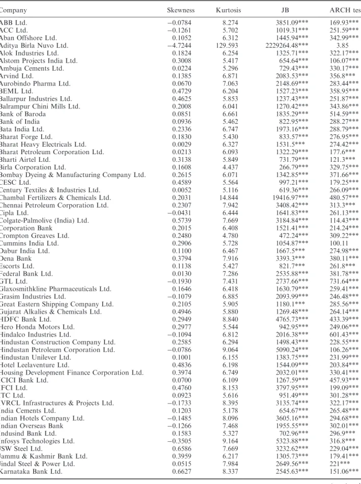
Table 1 reports the descriptive statistics for the log returns of each stock that is analysed. The table reports skewness, kurtosis, the Jarque–Bera (JB) test statistic (which examines the normality of the data) and the Lagrange Multiplier (LM) test (up to a lag of 12) of existence of heteroscedasticity by examining the presence of autocorrelation in squared residuals (Engle, 1982). The results indicate that the log returns series is mostly positively skewed and leptokurtic, thus violating the assumption of normal distribution.
This result is further confirmed by the JB test, which finds that the return, on all the stocks in the sample, is not normally distributed. The results of the LM test reveal that, in the case of all but three stocks, the squared return series was found to be auto correlated.
This hints a significant nonlinear temporal depen- dence and suggests that volatility may be following one of the ARCH-type processes. In summary, based on descriptive statistics, in all the stocks analysed, return volatility seems conditional and it changes over time.
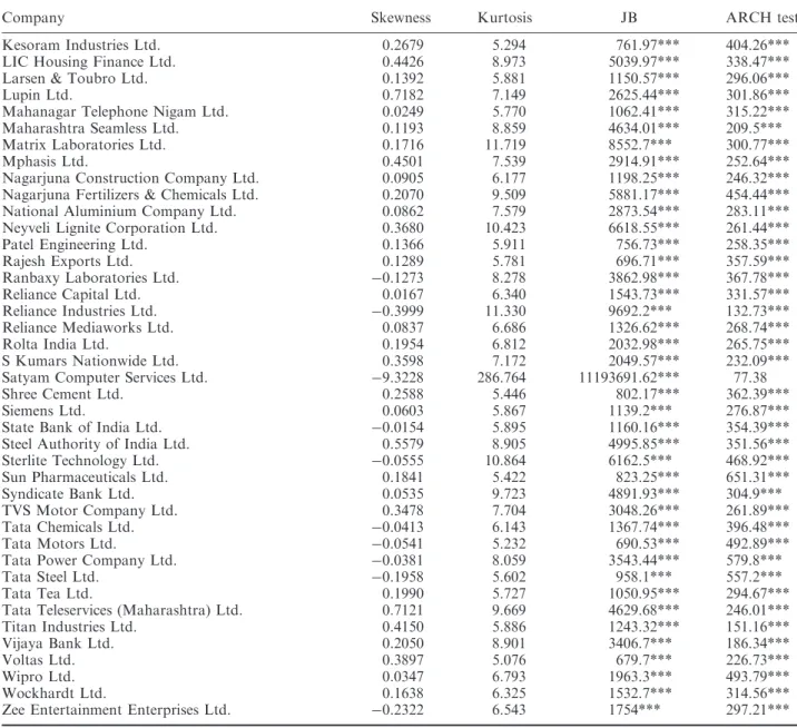
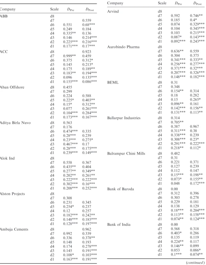
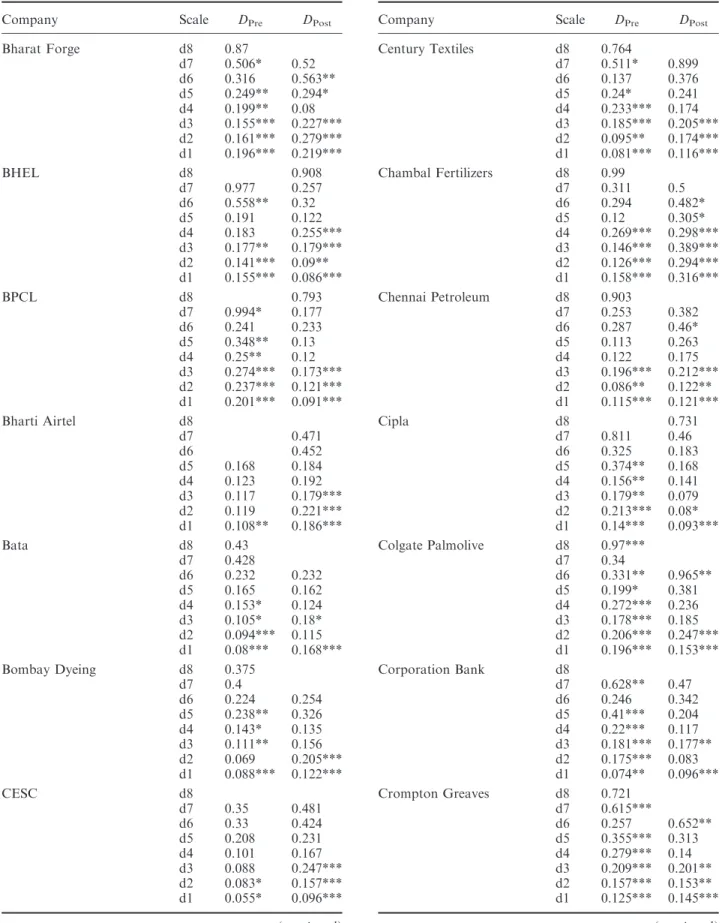
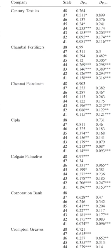
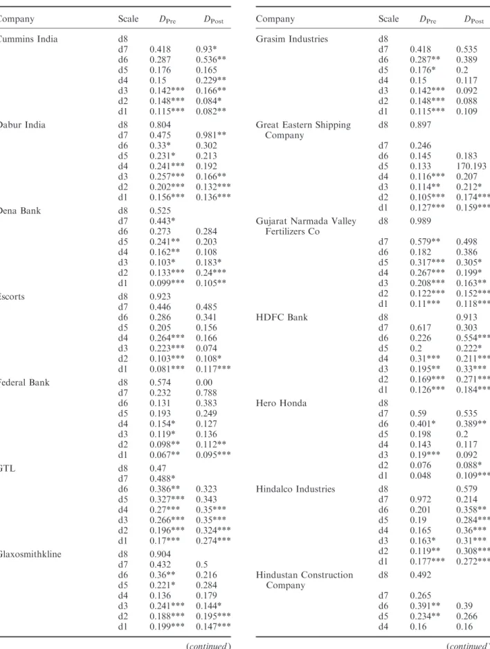
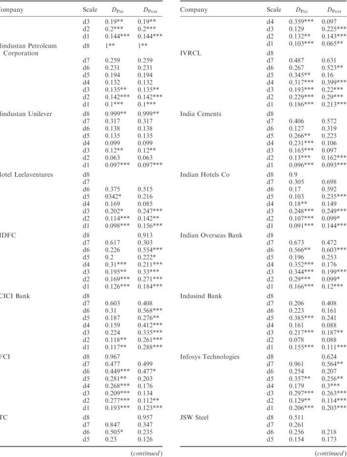
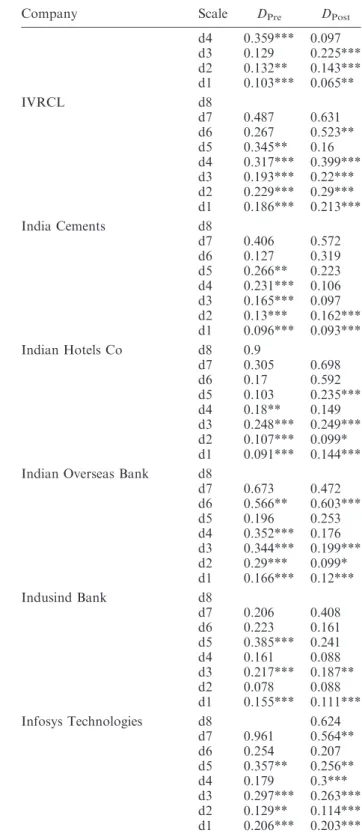
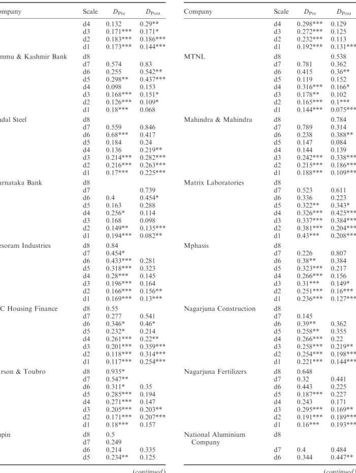
Before proceeding to model, the structure of conditional volatility in the pre- and post-derivative trading regimes, this article examines whether there exists a structural change around the time of intro- duction of derivatives trading following the wavelet variance analysis approach. This approach tells us the frequency at which there exist break points (discon- tinuity) in the conditional volatility series. The null hypothesis is that the variance is homogenous at each time scale (lower time scales such as d1, d2 and d3 and higher time scales such as d5, d6 and d7). The lower and higher time scales indicate short- and long- term volatility dynamics, respectively. The pattern of volatility break points in the pre- and post-derivatives trading regimes is compared to examine possible change in structure of stock return volatility around the time when derivatives trading is introduced on the underlying stock.
As reported in Table 2 (and summarized in Fig. 1), about 75% of the stocks experienced some change in the pattern of volatility between the two regimes. In the case of 28 companies’ stocks, volatility is found to be dynamic in short term in the pre-derivatives regime, while in the post-derivatives regime, volatility is seen to be dynamic in both the short as well as long term. In the case of 48 companies’ stocks, volatility is seen to be dynamic in the short as well as long term in the pre-derivatives regime while it is dynamic only in the short term in the post-derivative regime. In the
Table 1. Summary statistics of stock returns
Company Skewness Kurtosis JB ARCH test
ABB Ltd. 0.0784 8.274 3851.09*** 169.93***
ACC Ltd. 0.1261 5.702 1019.31*** 251.59***
Aban Offshore Ltd. 0.1052 6.312 1445.94*** 342.99***
Aditya Birla Nuvo Ltd. 4.7244 129.593 2229264.48*** 3.85
Alok Industries Ltd. 0.1824 6.254 1325.71*** 322.17***
Alstom Projects India Ltd. 0.3008 5.417 654.64*** 106.07***
Ambuja Cements Ltd. 0.0224 5.296 729.43*** 330.17***
Arvind Ltd. 0.1385 6.871 2083.53*** 356.8***
Aurobindo Pharma Ltd. 0.0670 7.063 2148.69*** 283.44***
BEML Ltd. 0.4729 6.204 1527.23*** 358.95***
Ballarpur Industries Ltd. 0.4625 5.853 1237.43*** 251.87***
Balrampur Chini Mills Ltd. 0.2008 6.041 1270.42*** 343.86***
Bank of Baroda 0.0851 6.661 1835.29*** 514.59***
Bank of India 0.0936 5.462 822.95*** 288.27***
Bata India Ltd. 0.2336 6.747 1973.16*** 288.79***
Bharat Forge Ltd. 0.1830 5.430 833.57*** 276.95***
Bharat Heavy Electricals Ltd. 0.0029 6.327 1531.5*** 274.42***
Bharat Petroleum Corporation Ltd. 0.0213 6.093 1322.29*** 177.6***
Bharti Airtel Ltd. 0.3138 5.849 731.79*** 121.3***
Birla Corporation Ltd. 0.1608 4.437 266.79*** 329.75***
Bombay Dyeing & Manufacturing Company Ltd. 0.2615 6.071 1342.85*** 371.66***
CESC Ltd. 0.4589 5.564 997.21*** 179.25***
Century Textiles & Industries Ltd. 0.0052 5.116 619.36*** 266.09***
Chambal Fertilizers & Chemicals Ltd. 0.2031 14.844 19416.97*** 480.57***
Chennai Petroleum Corporation Ltd. 0.2307 7.942 3408.42*** 313.3***
Cipla Ltd. 0.0431 6.444 1641.83*** 261.13***
Colgate-Palmolive (India) Ltd. 0.5739 7.669 3184.84*** 114.43***
Corporation Bank 0.2015 6.408 1521.41*** 214.24***
Crompton Greaves Ltd. 0.2480 4.780 472.24*** 309.22***
Cummins India Ltd. 0.2906 5.728 1054.87*** 100.11
Dabur India Ltd. 0.1100 6.467 1667.5*** 274.98***
Dena Bank 0.3794 7.916 3393.3*** 380.11***
Escorts Ltd. 0.1138 5.427 821.7*** 261.8***
Federal Bank Ltd. 0.0130 7.286 2535.88*** 381.78***
GTL Ltd. 0.1930 7.431 2737.66*** 731.64***
Glaxosmithkline Pharmaceuticals Ltd. 0.1646 6.418 1630.79*** 259.41***
Grasim Industries Ltd. 0.1079 6.885 2093.99*** 246.48***
Great Eastern Shipping Company Ltd. 0.2105 5.905 1180.1*** 285.56***
Gujarat Alkalies & Chemicals Ltd. 0.4946 5.880 1269.48*** 264.14***
HDFC Bank Ltd. 0.2949 8.840 4765.73*** 433.39***
Hero Honda Motors Ltd. 0.2977 5.544 942.95*** 249.06***
Hindalco Industries Ltd. 0.1094 6.812 2016.38*** 601.43***
Hindustan Construction Company Ltd. 0.2585 6.294 1498.43*** 228.55***
Hindustan Petroleum Corporation Ltd. 0.0786 9.064 5090.24*** 106.26***
Hindustan Unilever Ltd. 0.1001 6.155 1383.75*** 231.99***
Hotel Leelaventure Ltd. 0.4836 6.198 1544.09*** 203.84***
Housing Development Finance Corporation Ltd. 0.3974 6.749 2032.01*** 330.41***
ICICI Bank Ltd. 0.0700 6.109 1267.59*** 457.93***
IFCI Ltd. 0.4760 8.153 3797.95*** 199.09***
ITC Ltd. 0.0923 5.616 951.49*** 301.28***
IVRCL Infrastructures & Projects Ltd. 0.1733 8.395 3135.74*** 322.17***
India Cements Ltd. 0.1203 5.178 654.67*** 265.48***
Indian Hotels Company Ltd. 0.1485 8.096 3605.16*** 294.68***
Indian Overseas Bank 0.1266 7.468 1955.55*** 302.01***
Indusind Bank Ltd. 0.1583 5.327 702.96*** 296.9***
Infosys Technologies Ltd. 0.3505 9.164 5323.88*** 316.8***
JSW Steel Ltd. 0.6586 7.669 3232.62*** 229.04***
Jammu & Kashmir Bank Ltd. 0.3959 6.217 1305.73*** 179.41***
Jindal Steel & Power Ltd. 0.0515 7.984 2649.56*** 221***
Karnataka Bank Ltd. 0.6627 8.337 2545.63*** 151.06***
(continued)
case of about 25 companies’ stocks, no significant change in pattern of volatility is witnessed between the two regimes.
In summary, in most cases (76 out of 101), there seems to be a change in the structure of conditional volatility in the pre- and post-derivative regime.
Subsequently, in order to analyse the structure of conditional volatility, three alternative switching asymmetric GARCH (1, 1) specifications are
evaluated. These models make the stock return vola- tility conditional on ‘old’ and ‘new’ information, allowing for asymmetric response to ‘good’ and ‘bad’
news, for the two regimes. Figure 4 reports the NIC for the three models stated above for each stock analysed.
A flow chart of the process followed to arrive t the correct SAGARCH (1, 1) specification is given in Fig. 2. Also, an illustrative case has been discussed at the beginning of Fig. 4.
Table 1. Continued
Company Skewness Kurtosis JB ARCH test
Kesoram Industries Ltd. 0.2679 5.294 761.97*** 404.26***
LIC Housing Finance Ltd. 0.4426 8.973 5039.97*** 338.47***
Larsen & Toubro Ltd. 0.1392 5.881 1150.57*** 296.06***
Lupin Ltd. 0.7182 7.149 2625.44*** 301.86***
Mahanagar Telephone Nigam Ltd. 0.0249 5.770 1062.41*** 315.22***
Maharashtra Seamless Ltd. 0.1193 8.859 4634.01*** 209.5***
Matrix Laboratories Ltd. 0.1716 11.719 8552.7*** 300.77***
Mphasis Ltd. 0.4501 7.539 2914.91*** 252.64***
Nagarjuna Construction Company Ltd. 0.0905 6.177 1198.25*** 246.32***
Nagarjuna Fertilizers & Chemicals Ltd. 0.2070 9.509 5881.17*** 454.44***
National Aluminium Company Ltd. 0.0862 7.579 2873.54*** 283.11***
Neyveli Lignite Corporation Ltd. 0.3680 10.423 6618.55*** 261.44***
Patel Engineering Ltd. 0.1366 5.911 756.73*** 258.35***
Rajesh Exports Ltd. 0.1289 5.781 696.71*** 357.59***
Ranbaxy Laboratories Ltd. 0.1273 8.278 3862.98*** 367.78***
Reliance Capital Ltd. 0.0167 6.340 1543.73*** 331.57***
Reliance Industries Ltd. 0.3999 11.330 9692.2*** 132.73***
Reliance Mediaworks Ltd. 0.0837 6.686 1326.62*** 268.74***
Rolta India Ltd. 0.1954 6.812 2032.98*** 265.75***
S Kumars Nationwide Ltd. 0.3598 7.172 2049.57*** 232.09***
Satyam Computer Services Ltd. 9.3228 286.764 11193691.62*** 77.38
Shree Cement Ltd. 0.2588 5.446 802.17*** 362.39***
Siemens Ltd. 0.0603 5.867 1139.2*** 276.87***
State Bank of India Ltd. 0.0154 5.895 1160.16*** 354.39***
Steel Authority of India Ltd. 0.5579 8.905 4995.85*** 351.56***
Sterlite Technology Ltd. 0.0555 10.864 6162.5*** 468.92***
Sun Pharmaceuticals Ltd. 0.1841 5.422 823.25*** 651.31***
Syndicate Bank Ltd. 0.0535 9.723 4891.93*** 304.9***
TVS Motor Company Ltd. 0.3478 7.704 3048.26*** 261.89***
Tata Chemicals Ltd. 0.0413 6.143 1367.74*** 396.48***
Tata Motors Ltd. 0.0541 5.232 690.53*** 492.89***
Tata Power Company Ltd. 0.0381 8.059 3543.44*** 579.8***
Tata Steel Ltd. 0.1958 5.602 958.1*** 557.2***
Tata Tea Ltd. 0.1990 5.727 1050.95*** 294.67***
Tata Teleservices (Maharashtra) Ltd. 0.7121 9.669 4629.68*** 246.01***
Titan Industries Ltd. 0.4150 5.886 1243.32*** 151.16***
Vijaya Bank Ltd. 0.2050 8.901 3406.7*** 186.34***
Voltas Ltd. 0.3897 5.076 679.7*** 226.73***
Wipro Ltd. 0.0347 6.793 1963.3*** 493.79***
Wockhardt Ltd. 0.1638 6.325 1532.7*** 314.56***
Zee Entertainment Enterprises Ltd. 0.2322 6.543 1754*** 297.21***
Notes: The Kurtosis reported in the table is in excess of three.
The JB test statistic is calculated as: JB¼T 6
^
s2þðk^3Þ2 4
A2ð2Þ, where,Tis the total number of observations,s^the sample skewness andk^the sample kurtosis. LM is the Lagrange Multiplier test for ARCH effects (Engle, 1982), up to a lag of 12. The test statistic is again distributed as2ð12Þ.
Only thep-values are reported.
*** Indicates test statistic significance at 1% level.
Table 2. Wavelet variance analysis to detect volatility shifts at different time scales
Company Scale DPre DPost
ABB d8
d7 0.559
d6 0.551 0.68***
d5 0.249 0.184
d4 0.335** 0.136 d3 0.146 0.214***
d2 0.225*** 0.216***
d1 0.171*** 0.17***
ACC d8 0.923
d7 0.999** 0.459 d6 0.375 0.312*
d5 0.145 0.213*
d4 0.175 0.189**
d3 0.183** 0.194***
d2 0.096 0.135***
d1 0.155*** 0.086***
Aban Offshore d8 0.455
d7 0.299
d6 0.224 0.588
d5 0.225* 0.403**
d4 0.15* 0.312**
d3 0.077 0.261***
d2 0.104*** 0.284***
d1 0.173*** 0.167***
Aditya Birla Nuvo d8 0.563 d7 0.176
d6 0.474*** 0.335 d5 0.28*** 0.239 d4 0.23*** 0.275*
d3 0.467*** 0.17 d2 0.28*** 0.175***
d1 0.239*** 0.149***
Alok Ind d8
d7 0.558 0.367
d6 0.435** 0.404 d5 0.277** 0.349**
d4 0.202** 0.261**
d3 0.222*** 0.222***
d2 0.302*** 0.16***
d1 0.208*** 0.252***
Alston Projects d8
d7 0.308
d6 0.231 0.345
d5 0.254* 0.237
d4 0.12 0.257
d3 0.182*** 0.242**
d2 0.148*** 0.185***
d1 0.128*** 0.197***
Ambuja Cements d8 0.962
d7 0.992 0.339
d6 0.336 0.378**
d5 0.148 0.193
d4 0.174 0.278***
d3 0.145 0.191***
d2 0.108* 0.103***
d1 0.163*** 0.191***
Table 2. Continued
Company Scale DPre DPost
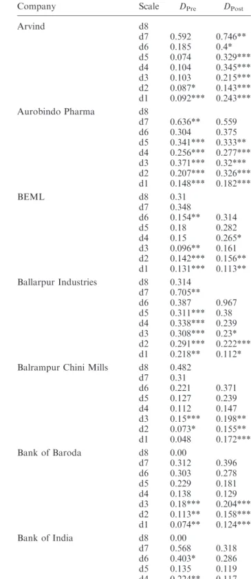
Arvind d8
d7 0.592 0.746**
d6 0.185 0.4*
d5 0.074 0.329***
d4 0.104 0.345***
d3 0.103 0.215***
d2 0.087* 0.143***
d1 0.092*** 0.243***
Aurobindo Pharma d8
d7 0.636** 0.559
d6 0.304 0.375
d5 0.341*** 0.333**
d4 0.256*** 0.277***
d3 0.371*** 0.32***
d2 0.207*** 0.326***
d1 0.148*** 0.182***
BEML d8 0.31
d7 0.348
d6 0.154** 0.314
d5 0.18 0.282
d4 0.15 0.265*
d3 0.096** 0.161 d2 0.142*** 0.156**
d1 0.131*** 0.113**
Ballarpur Industries d8 0.314 d7 0.705**
d6 0.387 0.967
d5 0.311*** 0.38 d4 0.338*** 0.239 d3 0.308*** 0.23*
d2 0.291*** 0.222***
d1 0.218** 0.112*
Balrampur Chini Mills d8 0.482
d7 0.31
d6 0.221 0.371
d5 0.127 0.239
d4 0.112 0.147
d3 0.15*** 0.198**
d2 0.073* 0.155**
d1 0.048 0.172***
Bank of Baroda d8 0.00
d7 0.312 0.396
d6 0.303 0.278
d5 0.229 0.181
d4 0.138 0.129
d3 0.18*** 0.204***
d2 0.113** 0.158***
d1 0.074** 0.124***
Bank of India d8 0.00
d7 0.568 0.318
d6 0.403* 0.286
d5 0.135 0.119
d4 0.224** 0.117 d3 0.146** 0.099 d2 0.053 0.086*
d1 0.1*** 0.074**
(continued)
Table 2. Continued
Company Scale DPre DPost
Bharat Forge d8 0.87
d7 0.506* 0.52 d6 0.316 0.563**
d5 0.249** 0.294*
d4 0.199** 0.08 d3 0.155*** 0.227***
d2 0.161*** 0.279***
d1 0.196*** 0.219***
BHEL d8 0.908
d7 0.977 0.257
d6 0.558** 0.32
d5 0.191 0.122
d4 0.183 0.255***
d3 0.177** 0.179***
d2 0.141*** 0.09**
d1 0.155*** 0.086***
BPCL d8 0.793
d7 0.994* 0.177
d6 0.241 0.233
d5 0.348** 0.13 d4 0.25** 0.12 d3 0.274*** 0.173***
d2 0.237*** 0.121***
d1 0.201*** 0.091***
Bharti Airtel d8
d7 0.471
d6 0.452
d5 0.168 0.184
d4 0.123 0.192
d3 0.117 0.179***
d2 0.119 0.221***
d1 0.108** 0.186***
Bata d8 0.43
d7 0.428
d6 0.232 0.232
d5 0.165 0.162
d4 0.153* 0.124 d3 0.105* 0.18*
d2 0.094*** 0.115 d1 0.08*** 0.168***
Bombay Dyeing d8 0.375
d7 0.4
d6 0.224 0.254
d5 0.238** 0.326 d4 0.143* 0.135 d3 0.111** 0.156 d2 0.069 0.205***
d1 0.088*** 0.122***
CESC d8
d7 0.35 0.481
d6 0.33 0.424
d5 0.208 0.231
d4 0.101 0.167
d3 0.088 0.247***
d2 0.083* 0.157***
d1 0.055* 0.096***
(continued)
Table 2. Continued
Company Scale DPre DPost
Century Textiles d8 0.764
d7 0.511* 0.899
d6 0.137 0.376
d5 0.24* 0.241
d4 0.233*** 0.174 d3 0.185*** 0.205***
d2 0.095** 0.174***
d1 0.081*** 0.116***
Chambal Fertilizers d8 0.99
d7 0.311 0.5
d6 0.294 0.482*
d5 0.12 0.305*
d4 0.269*** 0.298***
d3 0.146*** 0.389***
d2 0.126*** 0.294***
d1 0.158*** 0.316***
Chennai Petroleum d8 0.903
d7 0.253 0.382
d6 0.287 0.46*
d5 0.113 0.263
d4 0.122 0.175
d3 0.196*** 0.212***
d2 0.086** 0.122**
d1 0.115*** 0.121***
Cipla d8 0.731
d7 0.811 0.46
d6 0.325 0.183
d5 0.374** 0.168 d4 0.156** 0.141 d3 0.179** 0.079 d2 0.213*** 0.08*
d1 0.14*** 0.093***
Colgate Palmolive d8 0.97***
d7 0.34
d6 0.331** 0.965**
d5 0.199* 0.381 d4 0.272*** 0.236 d3 0.178*** 0.185 d2 0.206*** 0.247***
d1 0.196*** 0.153***
Corporation Bank d8
d7 0.628** 0.47
d6 0.246 0.342
d5 0.41*** 0.204 d4 0.22*** 0.117 d3 0.181*** 0.177**
d2 0.175*** 0.083 d1 0.074** 0.096***
Crompton Greaves d8 0.721
d7 0.615***
d6 0.257 0.652**
d5 0.355*** 0.313 d4 0.279*** 0.14 d3 0.209*** 0.201**
d2 0.157*** 0.153**
d1 0.125*** 0.145***
(continued)
Table 2. Continued
Company Scale DPre DPost
Cummins India d8
d7 0.418 0.93*
d6 0.287 0.536**
d5 0.176 0.165
d4 0.15 0.229**
d3 0.142*** 0.166**
d2 0.148*** 0.084*
d1 0.115*** 0.082**
Dabur India d8 0.804
d7 0.475 0.981**
d6 0.33* 0.302
d5 0.231* 0.213 d4 0.241*** 0.192 d3 0.257*** 0.166**
d2 0.202*** 0.132***
d1 0.156*** 0.136***
Dena Bank d8 0.525
d7 0.443*
d6 0.273 0.284
d5 0.241** 0.203 d4 0.162** 0.108 d3 0.103* 0.183*
d2 0.133*** 0.24***
d1 0.099*** 0.105**
Escorts d8 0.923
d7 0.446 0.485
d6 0.286 0.341
d5 0.205 0.156
d4 0.264*** 0.166 d3 0.223*** 0.074 d2 0.103*** 0.108*
d1 0.081*** 0.117***
Federal Bank d8 0.574 0.00
d7 0.232 0.788
d6 0.131 0.383
d5 0.193 0.249
d4 0.154* 0.127 d3 0.119* 0.136 d2 0.098** 0.112**
d1 0.067** 0.095***
GTL d8 0.47
d7 0.488*
d6 0.386** 0.323 d5 0.327*** 0.343 d4 0.27*** 0.35***
d3 0.266*** 0.35***
d2 0.196*** 0.324***
d1 0.17*** 0.274***
Glaxosmithkline d8 0.904
d7 0.432 0.5
d6 0.36** 0.216 d5 0.221* 0.284
d4 0.136 0.179
d3 0.241*** 0.144*
d2 0.188*** 0.195***
d1 0.199*** 0.147***
(continued)
Table 2. Continued
Company Scale DPre DPost
Grasim Industries d8
d7 0.418 0.535
d6 0.287** 0.389 d5 0.176* 0.2
d4 0.15 0.117
d3 0.142*** 0.092 d2 0.148*** 0.088 d1 0.115*** 0.109 Great Eastern Shipping
Company
d8 0.897 d7 0.246
d6 0.145 0.183
d5 0.133 170.193 d4 0.116*** 0.207 d3 0.114** 0.212*
d2 0.105*** 0.174***
d1 0.127*** 0.159***
Gujarat Narmada Valley Fertilizers Co
d8 0.989
d7 0.579** 0.498
d6 0.182 0.386
d5 0.317*** 0.305*
d4 0.267*** 0.199*
d3 0.208*** 0.163**
d2 0.122*** 0.152***
d1 0.11*** 0.118***
HDFC Bank d8 0.913
d7 0.617 0.303
d6 0.226 0.554***
d5 0.2 0.222*
d4 0.31*** 0.211***
d3 0.195** 0.33***
d2 0.169*** 0.271***
d1 0.126*** 0.184***
Hero Honda d8
d7 0.59 0.535
d6 0.401* 0.389**
d5 0.198 0.2
d4 0.143 0.117
d3 0.19*** 0.092 d2 0.076 0.088*
d1 0.048 0.109***
Hindalco Industries d8 0.579
d7 0.972 0.214
d6 0.201 0.358**
d5 0.19 0.284***
d4 0.165 0.36***
d3 0.163* 0.31***
d2 0.119** 0.308***
d1 0.177*** 0.272***
Hindustan Construction Company
d8 0.492 d7 0.265
d6 0.391** 0.39 d5 0.234** 0.266
d4 0.16 0.16
(continued)
Table 2. Continued
Company Scale DPre DPost
d3 0.19** 0.19**
d2 0.2*** 0.2***
d1 0.144*** 0.144***
Hindustan Petroleum Corporation
d8 1** 1**
d7 0.259 0.259
d6 0.231 0.231
d5 0.194 0.194
d4 0.132 0.132
d3 0.135** 0.135**
d2 0.142*** 0.142***
d1 0.1*** 0.1***
Hindustan Unilever d8 0.999** 0.999**
d7 0.317 0.317
d6 0.138 0.138
d5 0.135 0.135
d4 0.099 0.099
d3 0.12** 0.12**
d2 0.063 0.063
d1 0.097*** 0.097***
Hotel Leelaventures d8 d7
d6 0.375 0.515
d5 0342* 0.216
d4 0.169 0.085
d3 0.202* 0.247***
d2 0.114*** 0.142**
d1 0.098*** 0.156***
HDFC d8 0.913
d7 0.617 0.303
d6 0.226 0.554***
d5 0.2 0.222*
d4 0.31*** 0.211***
d3 0.195** 0.33***
d2 0.169*** 0.271***
d1 0.126*** 0.184***
ICICI Bank d8
d7 0.603 0.408
d6 0.31 0.568***
d5 0.187 0.276**
d4 0.159 0.412***
d3 0.224 0.335***
d2 0.118** 0.261***
d1 0.117** 0.288***
IFCI d8 0.967
d7 0.477 0.499
d6 0.449*** 0.477*
d5 0.281** 0.203 d4 0.268*** 0.176 d3 0.209*** 0.134 d2 0.277*** 0.112**
d1 0.193*** 0.123***
ITC d8 0.957
d7 0.847 0.347
d6 0.505* 0.235
d5 0.23 0.126
(continued)
Table 2. Continued
Company Scale DPre DPost
d4 0.359*** 0.097 d3 0.129 0.225***
d2 0.132** 0.143***
d1 0.103*** 0.065**
IVRCL d8
d7 0.487 0.631
d6 0.267 0.523**
d5 0.345** 0.16 d4 0.317*** 0.399***
d3 0.193*** 0.22***
d2 0.229*** 0.29***
d1 0.186*** 0.213***
India Cements d8
d7 0.406 0.572
d6 0.127 0.319
d5 0.266** 0.223 d4 0.231*** 0.106 d3 0.165*** 0.097 d2 0.13*** 0.162***
d1 0.096*** 0.093***
Indian Hotels Co d8 0.9
d7 0.305 0.698
d6 0.17 0.592
d5 0.103 0.235***
d4 0.18** 0.149 d3 0.248*** 0.249***
d2 0.107*** 0.099*
d1 0.091*** 0.144***
Indian Overseas Bank d8
d7 0.673 0.472
d6 0.566** 0.603***
d5 0.196 0.253
d4 0.352*** 0.176 d3 0.344*** 0.199***
d2 0.29*** 0.099*
d1 0.166*** 0.12***
Indusind Bank d8
d7 0.206 0.408
d6 0.223 0.161
d5 0.385*** 0.241
d4 0.161 0.088
d3 0.217*** 0.187**
d2 0.078 0.088
d1 0.155*** 0.111***
Infosys Technologies d8 0.624
d7 0.961 0.564**
d6 0.254 0.207
d5 0.357** 0.256**
d4 0.179 0.3***
d3 0.297*** 0.263***
d2 0.129** 0.114***
d1 0.206*** 0.203***
JSW Steel d8 0.511
d7 0.261
d6 0.256 0.218
d5 0.154 0.173
(continued)
Table 2. Continued
Company Scale DPre DPost
d4 0.132 0.29**
d3 0.171*** 0.171*
d2 0.183*** 0.186***
d1 0.173*** 0.144***
Jammu & Kashmir Bank d8
d7 0.574 0.83
d6 0.255 0.542**
d5 0.298** 0.437***
d4 0.098 0.153
d3 0.168*** 0.151*
d2 0.126*** 0.109*
d1 0.18*** 0.068
Jindal Steel d8
d7 0.559 0.846
d6 0.68*** 0.417
d5 0.184 0.24
d4 0.136 0.219**
d3 0.214*** 0.282***
d2 0.216*** 0.263***
d1 0.17*** 0.225***
Karnataka Bank d8
d7 0.739
d6 0.4 0.454*
d5 0.163 0.288
d4 0.256* 0.114
d3 0.168 0.098
d2 0.149** 0.135***
d1 0.194*** 0.082**
Kesoram Industries d8 0.84 d7 0.454*
d6 0.433*** 0.281 d5 0.318*** 0.323 d4 0.28*** 0.145 d3 0.196*** 0.164 d2 0.166*** 0.156**
d1 0.169*** 0.13***
LIC Housing Finance d8 0.55
d7 0.277 0.541
d6 0.346* 0.46*
d5 0.232* 0.214 d4 0.261*** 0.22**
d3 0.201*** 0.359***
d2 0.118*** 0.314***
d1 0.117*** 0.254***
Larson & Toubro d8 0.935*
d7 0.547**
d6 0.311* 0.35 d5 0.285*** 0.194 d4 0.271*** 0.147 d3 0.205*** 0.203**
d2 0.171*** 0.207***
d1 0.18*** 0.157
Lupin d8 0.5
d7 0.249
d6 0.214 0.335
d5 0.234** 0.125 (continued)
Table 2. Continued
Company Scale DPre DPost
d4 0.298*** 0.129 d3 0.272*** 0.125 d2 0.232*** 0.113 d1 0.192*** 0.131***
MTNL d8 0.538
d7 0.781 0.362
d6 0.415 0.36**
d5 0.119 0.152
d4 0.316*** 0.166*
d3 0.178** 0.102 d2 0.165*** 0.1***
d1 0.144*** 0.075***
Mahindra & Mahindra d8 0.784
d7 0.789 0.314
d6 0.238 0.388**
d5 0.147 0.084
d4 0.144 0.139
d3 0.242*** 0.338***
d2 0.215*** 0.186***
d1 0.188*** 0.109***
Matrix Laboratories d8
d7 0.523 0.611
d6 0.336 0.223
d5 0.322** 0.343*
d4 0.326*** 0.425***
d3 0.337*** 0.384***
d2 0.381*** 0.204***
d1 0.43*** 0.208***
Mphasis d8
d7 0.226 0.807
d6 0.38** 0.384 d5 0.323*** 0.217 d4 0.266*** 0.156 d3 0.31*** 0.149*
d2 0.251*** 0.16***
d1 0.236*** 0.127***
Nagarjuna Construction d8
d7 0.145
d6 0.39** 0.362 d5 0.258** 0.355 d4 0.266*** 0.22 d3 0.258*** 0.219**
d2 0.254*** 0.198***
d1 0.221*** 0.144***
Nagarjuna Fertilizers d8 0.648
d7 0.32 0.441
d6 0.443 0.225
d5 0.187*** 0.227
d4 0.243 0.171
d3 0.295*** 0.169**
d2 0.191*** 0.189***
d1 0.16*** 0.193***
National Aluminium Company
d8
d7 0.4 0.484
d6 0.344 0.447**
(continued)
Table 2. Continued
Company Scale DPre DPost
d5 0.295** 0.239*
d4 0.258*** 0.288***
d3 0.153** 0.262***
d2 0.114** 0.209***
d1 0.095*** 0.167***
Neyveli Lignite d8
d7 0.244 0.935**
d6 0.328 0.477**
d5 0.316** 0.278
d4 0.168 0.181
d3 0.333*** 0.223***
d2 0.251*** 0.188***
d1 0.33*** 0.239***
Patel Engineering d8
d7 0.303
d6 0.215 0.338
d5 0.122 0.207
d4 0.213** 0.251 d3 0.2*** 0.264***
d2 0.204*** 0.224***
d1 0.227*** 0.173***
Rajesh Exports d8
d7 0.51
d6 0.214 0.5
d5 0.293* 0.219 d4 0.417*** 0.227 d3 0.43*** 0.215**
d2 0.238*** 0.181***
d1 0.241*** 0.142***
Ranbaxy Laboratories d8 0.982
d7 0.884 0.384
d6 0.343 0.403**
d5 0.23 0.25**
d4 0.228* 0.392***
d3 0.237*** 0.256***
d2 0.292*** 0.275***
d1 0.31*** 0.279***
Reliance Capital d8 0.961
d7 0.536* 0.875 d6 0.205 0.576**
d5 0.33*** 0.278 d4 0.28*** 0.152 d3 0.183*** 0.255***
d2 0.187*** 0.187***
d1 0.126*** 0.16***
Reliance Industries d8 0.989
d7 1** 0.428
d6 0.323 0.425***
d5 0.199 0.143
d4 0.263** 0.199**
d3 0.146 0.334***
d2 0.106* 0.196***
d1 0.082* 0.145***
Reliance Media works d8
d7 0.261
d6 0.301 0.25
(continued)
Table 2. Continued
Company Scale DPre DPost
d5 0.163 0.269
d4 0.148 0.134
d3 0.138* 0.261***
d2 0.142*** 0.198***
d1 0.104*** 0.2***
Rolta India d8 0.405
d7 0.667***
d6 0.261 0.756**
d5 0.312*** 0.391*
d4 0.198*** 0.211 d3 0.25*** 0.228**
d2 0.225*** 0.204***
d1 0.17*** 0.153***
S Kumars d8
d7 0.649**
d6 0.256 0.497
d5 0.2 0.284
d4 0.135 0.264
d3 0.171*** 0.198***
d2 0.154*** 0.143***
d1 0.196*** 0.168***
Satyam Computer Services d8 0.606
d7 0.952 0.314
d6 0.342 0.498***
d5 0.177 0.651***
d4 0.145 0.739***
d3 0.19** 0.503***
d2 0.146*** 0.637***
d1 0.163*** 0.366***
Shree Cements d8 0.576
d7 0.678***
d6 0.222 0.473
d5 0.41*** 0.203 d4 0.276*** 0.204 d3 0.345*** 0.183*
d2 0.267*** 0.125 d1 0.279*** 0.121***
Siemens d8 0.66
d7 0.367 0.798
d6 0.429*** 0.571**
d5 0.214** 0.331**
d4 0.365*** 0.186 d3 0.267*** 0.127 d2 0.306*** 0.215***
d1 0.204*** 0.132***
State Bank of India d8 0.821
d7 0.554 0.186
d6 0.315 0.529***
d5 0.25 0.141
d4 0.258** 0.287***
d3 0.115 0.277***
d2 0.16*** 0.178***
d1 0.093** 0.145***
Steel Authority of India d8 0.625 d7 0.388
d6 0.23 0.465
(continued)
Table 2. Continued
Company Scale DPre DPost
d5 0.153 0.17
d4 0.297*** 0.123 d3 0.216*** 0.185**
d2 0.136*** 0.161***
d1 0.168*** 0.134***
Sterlite Technology d8
d7 0.337
d6 0.133 0.332
d5 0.323** 0.258 d4 0.266*** 0.231 d3 0.147** 0.209**
d2 0.176*** 0.228***
d1 0.112*** 0.22***
Sun Pharmaceuticals d8
d7 0.344 0.622
d6 0.459*** 0.337 d5 0.388*** 0.311*
d4 0.393*** 0.183 d3 0.366*** 0.253***
d2 0.264*** 0.112**
d1 0.198*** 0.158***
Syndicate Bank d8
d7 0.289
d6 0.65** 0.269 d5 0.426** 0.134 d4 0.414*** 0.147
d3 0.16 0.147**
d2 0.306*** 0.123***
d1 0.14*** 0.094***
TVS Motors d8
d7 0.23 0.488
d6 0.22 0.314
d5 0.125 0.356*
d4 0.186** 0.15 d3 0.138** 0.168**
d2 0.113*** 0.187***
d1 0.133*** 0.193***
Tata Chemicals d8 0.97
d7 0.436 0.509
d6 0.25 0.617***
d5 0.153 0.41***
d4 0.105 0.244**
d3 0.098 0.357***
d2 0.088** 0.261***
d1 0.132*** 0.21***
Tata Motors d8 0.585
d7 0.561 0.383
d6 0.37 0.717***
d5 0.174 0.103
d4 0.218* 0.253***
d3 0.163* 0.296***
d2 0.162*** 0.299***
d1 0.158*** 0.16***
Tata Power d8 0.994*
d7 0.923 0.502*
d6 0.305 0.425***
(continued)
Table 2. Continued
Company Scale DPre DPost
d5 0.234 0.203
d4 0.356*** 0.304***
d3 0.197** 0.258***
d2 0.254*** 0.196***
d1 0.197*** 0.189***
Tata Steel d8 0.998*
d7 0.602 0.251
d6 0.199 0.613***
d5 0.11 0.147
d4 0.182 0.327***
d3 0.129 0.351***
d2 0.144*** 0.216***
d1 0.146*** 0.231***
Tata Tea d8 0.992
d7 0.642 0.287
d6 0.32 0.235
d5 0.204 0.099
d4 0.156 0.156*
d3 0.085 0.085
d2 0.187*** 0.094**
d1 0.105*** 0.062**
Tata Teleservices d8
d7 0.339
d6 0.265 0.323
d5 0.26* 0.212
d4 0.119 0.168
d3 0.153*** 0.213**
d2 0.168*** 0.194***
d1 0.133*** 0.174***
Titan Industries d8 0.839
d7 0.334 0.434
d6 0.273 0.198
d5 0.113 0.2
d4 0.218*** 0.25**
d3 0.079 0.127
d2 0.078* 0.125**
d1 0.077*** 0.123***
Vijaya Bank d8
d7 0.827 0.8
d6 0.441 0.507**
d5 0.269 0.33**
d4 0.219* 0.197*
d3 0.247*** 0.21***
d2 0.213*** 0.106*
d1 0.072 0.131***
Voltas d8 0.758
d7 0.517**
d6 0.404*** 0.399 d5 0.282*** 0.358 d4 0.165*** 0.134 d3 0.226*** 0.166 d2 0.151*** 0.16**
d1 0.128*** 0.147***
Wipro d8
d7 0.487 0.3
d6 0.317 0.465**
(continued)
Accordingly, in the case of most of the companies’
stocks analysed (88 out of 101), a GJR GARCH model was found suitable. In most of these cases, the EGARCH specification was also appropriate, but the EGARCH model returned an unreasonably large conditional volatility for very ‘bad’ news (large negative values of "t1). Also, in such cases, the conditional volatility given by the EGARCH model remained more or less constant for ‘good’ news (positive values of "t1). Thus, in such cases, a GJR GARCH specification was preferred because it ade- quately captured response of volatility to both ‘good’
as well as ‘bad’ news. This finding is in conformity with Engle and Ng (1993) and Kim and Kon (1994), who find GJR GARCH to be a more appropriate specification among alternative asymmetric GARCH models. A PGARCH was found appropriate in the case of another 10 stocks and EGARCH in the case
of 3 stocks. Table 3 reports the results of the switching asymmetric GARCH specification of con- ditional volatility. An illustrative case is explained in the notes to Table 3. Relevant results from Table 3 are summarized in Fig. 3.
Based on Table 3 (summarized in Fig. 3), the following observations can be made:
(i) In more than 85% of the cases, the SAGARCH (1, 1) model was found to be a good fit. In other words, post fit there was no evidence of autocorrelation in the squared residuals.
(ii) The unconditional volatility for different switching asymmetric GARCH (1, 1) specifi- cations has increased in 60 of the 101 stocks analysed. Thus, hinting at an increase in the quantity of information flowing into the spot markets after introduction of derivatives trading.
(iii) In the case of 61 stocks, the asymmetric response is either reduced or removed com- pletely after introduction of derivatives trad- ing. In the case of another 22 stocks, the extent of asymmetry is more pronounced in the post- derivatives regime. In the case of 18 stocks, the introduction of derivatives trading does not seem to affect asymmetric response. Thus, if the asymmetric response was due to market imperfections, (reaction of noise traders as in Black (1986)), then in the case of more than 60% of the stocks analysed, the introduction of derivatives trading seems to have increased the information efficiency of the stock market.
(iv) The ‘news coefficient’ decreased in the case of 73 stocks. In other words, the introduction of derivative trading seems to have reduced the rate of absorption of ‘new’ information into spot prices.
(v) The ‘persistence coefficient’ has reduced in the case of all the stocks analysed. In other words, the impact of ‘old’ information on current volatility seems to have reduced.
Discussion
Based on the results, it can be said that while the introduction of derivatives trading has mostly reduced (and not removed) asymmetric response of volatility, it has also reduced the impact of ‘old’
information on stock prices, as well as the speed with which ‘new’ information is incorporated in prices.
At the outset, this sounds counter intuitive because theoretically, the reduction in spot market return volatility happens because of lower dependence on past volatility and higher rate at which ‘new’ infor- mation is being reflected in stock prices. To explain Table 2. Continued
Company Scale DPre DPost
d5 0.186 0.281**
d4 0.175 0.146
d3 0.145** 0.166***
d2 0.147*** 0.143***
d1 0.184*** 0.098***
Wockhardt d8
d7 0.365 0.681
d6 0.426** 0.564**
d5 0.262** 0.362**
d4 0.226*** 0.247**
d3 0.365*** 0.203***
d2 0.215*** 0.182***
d1 0.209*** 0.257***
Zee Entertainment d8 0.499 d7 0.318
d6 0.301 0.551
d5 0.366* 0.249 d4 0.297*** 0.335**
d3 0.269*** 0.146 d2 0.228*** 0.225***
d1 0.181*** 0.171***
Note: ***,** and * indicate test statistic significance at 1, 5 and 10% levels, respectively.
Frequency at which there exists a structural break in volatility
Post derivatives Pre derivatives
Low High Low and high
Low 11 companies 0 28 companies
High 0 0
Low and high 48 companies 0 14 companies
Fig. 1. Summary of the wavelet variance analysis test results
this counter intuitive finding, let me start with an analysis of past studies that examine the said issue (Antoniou and Holmes, 1995; Bologna and Cavallo, 2002; Bandivadekar and Ghosh, 2003). Their conclu- sion that introduction of derivatives leads to a reduction in persistence (effect of ‘old’ information) due to an increase in rate of absorption of ‘new’
information is based on the following premises:
(i) Introduction of derivatives trading would lead the informed speculators as well as the noise traders to migrate to the derivative market,
thus creating a new set of active information seekers in this market.
(ii) Consequently, there would be a lot of infor- mation that is being generated in the deriva- tives market and then transmitted to the spot market.
(iii) Post migration of noise traders, the remaining investors would use this ‘new’ information to arrive at a fair price rapidly.
In reality, a lot depends on the quality of the information emanating from the derivatives market.
Input: Log return of sample stocks, NSE nifty index and a dummy variable which takes a value ‘0’ before trading in derivatives are introduced and ‘1’ after
Estimate 3 alternative SAGARCH (1, 1) specification of conditional volatility using quasi maximum likelihood estimation
Check the goodness-of-fit of each SAGARCH (1, 1) specification following LBTSSR and rank LBTSSR (See Table 3)
Check NIC for asymetric response as captured by SAGARCH (1, 1) specification that gives a good fit
Check if there exists more than one model which gives a good fit as well as captures
Start
Select the specification which gives minimum response of conditional volatility in the absence of
new information
End
Select the given model Bad
All 3 specifications are bad.
No Does not capture
asymmetry Good
At least one specification gives a good fit
Yes Captures asymmetry
No
Yes
Fig. 2. Flow chart for the process followed to select the (switching SAGARCH (1, 1)) asymmetric GARCH (1, 1) model of conditional volatility