IMPACT OF INFORMATION SHARING IN A MICRO CREDIT MARKET WITH GROWING POPULATION

IMPACT OF INFORMATION SHARING IN A MICRO CREDIT MARKET WITH GROWING POPULATION

Bhaswar Moitra^∗, Saswatee Mukherjee^∗∗, Saikat Sinha Roy^∗∗∗

Abstract

This paper presents how in a paradigm of asymmetric information, sharing of information among the lenders about their borrower types can turn out to be profitable, to lenders and borrowers alike, in a dynamic framework with growing population. The result identifies how heterogeneity within the borrower group reduces the interest rate faced by the disciplined (safe) ones. It also suggests that collusion among the lenders, via sharing of information about their defaulting borrowers, benefit them through increased profit. Apart from this, the paper shows that in a credit market with asymmetric information, a monopolist lender (without any capacity constraint) can offer credit at better terms than his competing counterparts.

JEL classification: G21; D83; D41

Keywords: MFIs; Information sharing; Competition; Monopoly

      

∗ Professor, Department of Economics, Jadavpur University. 

∗∗ Research Fellow, Department of Economics, Jadavpur University. 

∗∗∗ Reader, Department of Economics, Jadavpur University. 

This paper explores the role and impact of information sharing among the lenders under competitive market structure on the microcredit lending rates in a dynamic growing population framework. In doing so, we have also compared the results with a model of monopolist lender.

The framework of Grameen 2 (2000) model, which replaces group lending contract by individual lending, has been used in this analysis.

Rising competition among the lenders in the credit market has always been a cause for concern.

Contrary to the common perception that competition ensures efficiency, overcrowding of lenders in the credit market actually drives the market away from such a Pareto efficient state. This reversal of outcome can be attributed to the existence of adverse selection-moral hazard problem¹ which nullifies the efficacy of competition among the lenders by increasing the interest rate as well as the rate of repayment default. In this regard, it can be said that market with a monopoly lender rather improves the performance and profitability of the lender by reducing the threat of borrowers’ default which in turn results in the reduction of the interest rate imposed on the borrowers, thus aiding in disciplining the borrowers’ repayment schedule. This is evident in Kranton and Swamy (1999)². The monopoly lender, as a result, charges a comparatively low interest rate which has a cascading effect on the reduction of default rate. There is thus a downward spiraling effect between interest rate and rate of repayment default of the borrowers.

This increases the overall efficiency of the lending contract through welfare improvement of both lender and borrower involved in the contract.

In the presence of competition, with no entry-exit restrictions on the lenders in the credit market, the possibility of earning a supernormal profit attracts potential entrants to extract the surplus from the market and drive down the profit level. Microfinance is no exception. After its initial tranche of success period with the first movers enjoying a supernormal profit, many other institutions start overcrowding this niche market. With microcredit market being in its nascent stage, the new entrants also continued to earn a positive return on their investment. However, the supply-side reaches its state of saturation and the bubble bursts. Before the micro-finance institutions (MFIs) and the donor agencies apprehend the situation, the borrowers start double       

1 Stiglitz (2000) explained how perfect and complete information in the market can be a Pareto superior outcome over asymmetric information. 

2 Kranton and Swamy (1999) showed in the backdrop of colonial India how greater outreach of the moneylenders increased competition in the credit market and worsen the situation of the borrowers through welfare deterioration.

dipping (multiple loans)³ which automatically reduces their repayment rate. The MFIs react by increasing the interest rate to cover their costs of lending. In some cases, the MFIs also introduce compulsory savings programme to minimize their loss⁴ whereby the borrowers are required to maintain a savings account with the MFIs which in due course can be invoked as collateral in case of default. This results in increased financial obligations of the borrowers who in the process start defaulting all the more, while the lenders retaliate further by increasing the rate of interest. As a result, none of the parties (lenders or borrowers) benefit out of this, which made the donor agencies, vying for healthy return, refrain from investing money in this market⁵. Nevertheless, the core of this problem is that increased competition actually leads to the deviation of the MFIs from their operational philosophy of reducing social poverty through providing cheap credit to the poor⁶, who have no access to formal sector lending.

To address the above problems, the practitioners of microfinance and the policy makers came up with certain relief tool in the form of market sharing according to geographical⁷ as well as demographical selections⁸, dynamic incentive mechanism⁹, etc. Strikingly the most prominent among them is that of information sharing contract among the lenders through the formation of information sharing bureau. This concept of information sharing is strongly advocated by Stiglitz (2000)¹⁰ as a remedy tool in any paradigm of asymmetric information. Again, Pagano and Jappelli (1993) showed that the existence of the credit bureaux in situation of increasing competition with asymmetric information helps lenders to discipline the borrowers by regularizing their repayment schedule. Also with demographics characterized by high degree of mobility and improved technology, the availability of these bureaux can actually benefit the       

3 Vogelgesang (2001) showed in his empirical analysis that increased competition in the credit market leads to multiple borrowings, which automatically increases the default rate of the borrowers. 

4 Morduch (1999). 

5 Morduch (1999) and Morduch (2000), showed how the donor agencies create a subsidy trap for the MFIs whereby the efficiency of the lending institutions are reduced since they never become financially sustainable. Also due to increased competition in lending market, donor bodies are reluctant to advance subsidized credit to the MFIs owning to fear of default.

6 McIntosh and Wydick (2005) showed how competition among lenders in credit market reduces the rent from profitable borrowers thereby making credit expensive for the poorer clients.

7 McIntosh, Janvry, and Sadoulet (2005) in a survey done in Uganda, found how increased competition leads to the polarization of lenders spatially according to their types.

8 Andersen and Moller (2006) supported the coexistence of both formal and informal lenders catering to different clienteles with differential lending contracts with respect to collateral requirements and interest rates. Navajas, Conning, and Vega (2003) have found the same result in Bolivian microcredit market.

9 Besley and Coate (1995), Morduch (1999), and Tedeschi (2006). 

10 Stiglitz (2000) explained how perfect and complete information in the market can be a Pareto superior outcome over asymmetric information.

lenders as is found in UK, US, Japan etc¹¹. Thus, the existence of these bureaux is a natural monopoly but it is discouraged by the threat of the potential entrants in the credit market. It is seen that fresh entrants might disturb the information sharing agreements among the existing lenders thereby making the bureau unstable.

This entire benefit of information sharing can be ascribed to the reputation effect that it imparts.

In a different context, Greif (1993) showed how using merchant laws and endogenous information sharing through the formation of trading groups, the overseas trade relations can be controlled by the merchants. It was found that any overseas trader, who cheats any member of the trading group, loses all future contracts with the others of the same group. On the contrary, the time length of the information shared by the lenders can have a negative impact on this reputation effect. Vercammen (1995) showed that too out-dated credit history of any borrower can increase his incentive to take up risky project that might reduce the welfare of the lenders through reduction in reputation effect. A similar indication has been found in the works of Padilla and Pagano (1997), and Padilla and Pagano (2000) where informational monopoly of the banks has a reverse impact on the reputational threat on the safe type borrowers whereby they are reluctant to put optimal effort level, thus reducing the project return. Hence it is said that sharing partial black (past defaults) information about the borrowers is better than signaling the entire credit history i.e. black and white (current debt exposure, performance and riskiness) information about them. Also one-shot lending contracts (single period) necessitates information sharing among the lenders, the urge of which becomes feeble with multi-period lending involving relationship banking [Brown and Zehnder (2005)]. However in a duopolistic market, it is found that lenders sharing information about their borrower types always head to an increase in the surplus generated by them [Vives (1990) , Malueg and Tsutsui (1996)].

In this paper we have tried to analyse the impact of information sharing among the lenders under competitive framework on the lending rates. The model that follows differs from the ones mentioned above, in a way that here we considered a changing demography/growing population under a multi period framework. In the literature we can find that even the worst type of borrowers can be disciplined with a custom-made interest rate structure, which will force them to

      

11 Jappelli and Pagano (2002). 

self-select¹² under different market scenarios. In addition to this, such self-selection by the borrowers can be reinforced by a well functioning information sharing contract among the lenders. Apart from that, the existence of the risky types of borrowers in the credit market helps the lenders to derive monopoly rent from them, which in turn reduces the interest rate faced by the safer ones; a result quite opposite to that of Akerlof’s lemons problem. Moreover, it is shown how the existence of a monopoly lender in this niche market with asymmetric information can be welfare enhancing for the target group of poor borrowers over credit market catered by many competing lenders. This result fits well into the predictions by Kranton and Swamy (1999). The paper is organized as follows. In section 1, we present a dynamic multi-period model without information sharing under monopolistic and competitive paradigm. In section 2, we consider model with information sharing among the lenders while in section 3, we conclude by summarizing the results.

1. THE BASIC MODEL WITH GROWING POPULATION (WITHOUT INFORMATION SHARING)

1.1 Single lender

Let us consider a basic principal-agent framework. There is a lender (principal) who lends L unit of capital to a borrower (agent) for which, he charges an interest rate r. The borrower then invests this capital in some project and realizes a return Y with probability (1−p) , and 0 otherwise, with 0≤ p≤1. p can thus be denoted as the probability of facing a shock. However after the output is realized, the borrower then decides whether to pay back the loan or not. Hence, we have a moral hazard problem here, where the borrower decides expost whether to deafult. Let us assume the borrower's probability of default to be θ, with 0≤θ≤1. Also let us assume that there are two types of borrowers in the market, safe and risky, whom the monopolist lender cannot discriminate before lending. Hence we have a problem of adverse selection also. Let θ_S and θ_R be the default probabilities for the safe and risky types of borrowers respectively where

S

R θ

θ > .

      

12 Mas-Colell, Whinston and Green (1995).

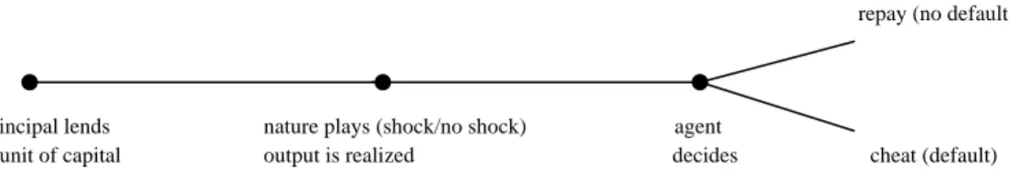
Hence the time line of the model can be written as follows:

repay (no default)

principal lends nature plays (shock/no shock) agent

L unit of capital output is realized decides cheat (default)

Fig 1: The time line of the lending contract between a monopoly lender (principal) and the borrower (agent).

Here we take the initial population to be N out of which for simplicicity 2

N are assumed to be

of safer types, while the remaining 2

N are the risky types. To accomodate demographic dynamism in this model, we assume the population to grow at a rate of k fraction of the previous period population. 

Proposition 1: With a monopoly lender, the interest rate faced by the borrowers

reduces with their riskiness. i.e. dr

M

/dθ < 0, where, r

M

is the interest rate charged by the monopolist lender.

Proof: In this model, a borrower is expected to repay back his loan if, gain from cheating ≤ gain from repayment 

In other words,

[

− +

]

+ −

[

− +

]

+ −

[

− +

]

+ +∞

≤ Y L(1 r) (1 )Y L(1 r) ²(1 )²Y L(1 r) ...

Y δ θ δ θ

or,

[

(1 )

]

) (1 1

1 Y L r

Y − +

−

≤ −

δ θ or,

δ θ δ

θ 1 (1 )

) (1 )

(1 1 1 1

−

−

− +

⎥≤

⎦

⎢ ⎤

⎣

⎡

−

− − L r

Y

or, ^Y

[

^{1−(1−θ)δ−1}

]

^{≤−L(1+r)]}

or,

δ θ) (1

) (1

−

− +

≤ −L r Y

or,

δ θ) (1

) (1

−

≥ L +r

Y ...(1) where, δ is the discounting factor.

From the above equation (1), we can calculate the rate of return to be, L(1+r)≤Y(1−θ)δ

or, ≤ (1−θ)δ −1 L

r_M Y ...(2)

Thus we find that the higher the value of θ, the lower is the interest rate faced by the borrower.

Proposition 2: Existence of risky types in the market lowers the interest rate faced

by the safe types.

Since we have identified two types of borrowers in the market with different default probabilities, hence if the monopolist lender can actually offer different contracts for two types of borrowers, then the interest rates charged by the lender to each type would be,

_Mⁱ ≤ (1−θ_i)δ−1 L

r Y ...(3)

i=R,S refers to risky and safe types respectively.

Now putting both the interest rates as equality, we can compare the lending rates faced by both types of borrowers.

R M S

M r

r −  

1]

) (1 [ 1]

) (1 [

= − _S − − − _R −

L Y L

Y θ θ  

) 1 (1

= _{S R}

L

Y −θ − +θ  

If, θ_R >θ_S

0

>

) (

= _{R S}

L

Y θ −θ

R M S

M r

r >

⇒ ...(4)

A very interesting result can be concluded from the above- in an adverse selection-moral hazard lending contract with a single lender, the risky type borrower always enjoys a lower interest rate than his safe counterpart. This result is counter-intuitive to our general belief that the greater the riskiness of any borrower type, the higher is the lending rate faced by him¹³.

However, since the monopolist lender does not have any tool to identify his borrower type, he can offer the same contract to both types of borrowers with,

r_M =min[r_M^R,r_M^S]=r_M^R …...(5) Thus if the monopolist lender charges the above rate to all the borrowers unanimously irrespective of their types, then none of them will default and the lender will earn a lifetime positive return without bothering to identify the type of the borrowers. Also, considering the beak-even situation, the monopolist lender will always try to keep his interest rate within the following range where the term on the left hand side of the following equation (6) represents the break-even interest rate under monopolistic market¹⁴,

= (1 ) 1

) (2

)

( ≤ ≤ − −

−

−

+ θ δ

θ θ

θ θ

R R

M M S R

S R

L r Y

r ...(6)

1.2  Two identical competing lenders  

The basic framework of a competitive model is the same as that with a single lender, apart from the fact that here we have two identical lenders (lender A and lender B) operating in the same market whom the borrowers can borrow from. Any borrower can cheat a lender and reapply for credit from the second one. It is assumed in the model that the lenders do not have any information sharing arrangement between themselves. Hence neither of the lenders can ever       

13 Stiglitz and Weiss (1981), showed how presence of risky type of borrowers in the credit market puts an upward pressure on the interest rate charged by the lenders which gradually drives the safe borrowers out of the market.

14 See appendix A.1. 

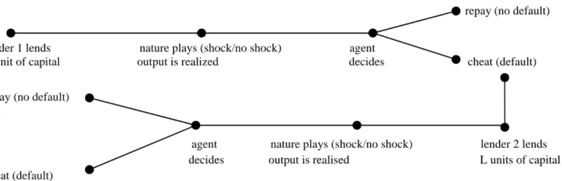
know the credit history of any of the borrowers unless once cheated by that borrower. Thereby any borrower can cheat each of the lenders only once after which, his history will be known to both the lenders. Thus, in total, any borrower will chance to cheat twice in this framework, once for each lender. To start with, the basic features of dynamism is preserved in this model. Hence the time line of the model can be composed as follows:

repay (no default)

lender 1 lends nature plays (shock/no shock) agent

L unit of capital output is realized decides cheat (default) repay (no default)

agent nature plays (shock/no shock) lender 2 lends decides output is realised L units of capital cheat (default)

Fig 2: The time line of the lending contract between two identical competiting lenders (principal) and the borrower (agent).

Proposition 3: With competing lenders offering no incentive schemes, the

borrowers, irrespective of their types, will always cheat their first lender.

Proof:   Under this competitive framework, any borrower will repay his loan if, repayment payoff ≥ payoff from cheating

In other words,

Y−L(1+r)≥Y+(1−θ)δ

[

Y−L(1+r)

]

+(1−θ)²δ²

[

Y−L(1+r)

]

+....+∞

or, 0≥L(1+r)+(1−θ)δ

[

Y−L(1+r)

]

+(1−θ)²δ²

[

Y−L(1+r)

]

+....+∞ ...(7)

Clearly the above inequality is an impossibility. Hence it can be concluded safely that with two competing lenders without any information sharing contract between themselves, borrowers will always choose to default in their first period of borrowing.

To address this problem, we can bring in microfinance institutions as a relief tool, who, by way of various social sanction methods, can guarantee the repayment by the borrowers even under a competitive framework. It is assumed that microfinance providers can induce a part of the

borrower group (safe types) through proper incentive provisioning in the form of reduced interest rates, future credit guarantee, increased credit volume¹⁵, etc to repay back their loan.

Our task now is to see how in this framework, the lenders equilibriates on their offered interest rates. To do this, let us assume two situations:

(i) r_A=r_B=r for the new borrowers and r_A =r_B =r^∗ =r−∈ for the old borrowers where ∈→0 (ii)r_A<r_B where r_A+α=r_B=r_M for the new borrowers with α→0 and r_M is the monopoly rate and r_A−β =r^∗ for the old borrowers where β →0

With r_A=r_B=r, the structure of market sharing between the lenders is as follows. In this case, since both the lenders charge the same interest rate, the borrowers are indifferent between the lenders while applying for credit. Hence both the lenders get equal share of the popualtion to lend to. Now in the 1^st period of lending, the total population is N , so both the lenders get to address

2

N number of borrowers. Going by the model, only the 4

N safe types of each lender

return their money while the 4

N risky types of both the lenders default. Hence the net payoff for each of the lenders is,

) )(1 4 (1

2 N L r ^S

N L+ + −θ

−

Proposition 4: Under dynamic population model with competition, none of the

lenders will be able to identify the types of the borrowers (fromamongst 2

^nd

period new applicants) ever, if they both charge the same interest rate .

In the 2^nd period of lending, the total population is N+kN =N(1+k). Hence the total number of new entrants in the market are kN. Thus each lender gets

4

N safer types of the 1^st period who are now old borrowers to him and whose credit history is known to respective lenders charging       

15Besley and Coate (1995), Morduch (1999), and Tedeschi (2006) showed how dynamic incentive schemes can be used as collateral substitutes in presence of adverse selection to discipline borrowers and reduce their probability of strategic default.  

them an interest rate r^∗. Since these borrowers are by nature the safe types, they will continue to be safe in this period and repay their loan. As with the new applicants approaching each lender, there are

4

N risky types migrating from the other lenders of the 1^st period as well as 2

kN new entrants of the 2^nd period. Since we can see that neither of the lenders can segregate between the fresh entrants and the 1^st period defaulting migrants, each lender being handicapped by this informational asymmetry has to treat both the above fractions (defaulting migrants and new entrants) as of same entity and charge them a uniform rate as applicable on the new borrowers.

However, out of them, the migrants who have already defaulted with their 1^st period lender and will not get access to either of the credit windows subsequently if they continue to cheat in this period also. Hence the migrants, although risky by nature, will repay their loan. As regards with the new entrants, safer half will repay their loan while the risky half will by their nature cheat.

Thus the net payoff of each of the lenders stands at,

) )(1 4 (1

) )(1 4 (1

) )(1 4 (1

2 ] 4

[4 _{S R} kN L r _S

r N L

r N L

kN L N

N + + + + −θ + + −θ + + −θ

− ^∗

In the 3^rd period, the total population is (N+kN)(1+k)=N(1+k)². Out of these, N are from the 1^st period, kN from the 2^nd period and there are k(1+k)N new entrants in the 3^rd period.

Thus each lender gets 2

N (all safe now) from the 1^st period, 4

kN safe types from the 2^nd period as old and known customers, to both of whom, each charges r^∗and gets back his return with certainity. As with the new borrowers coming to each lender, there are

4

kN risky types of the

other lender from the 2^nd period and 2

) (1 k N k +

freshers of the 3^rd period. Once again, the lenders cannot discriminate between them and treat them alike, charging all of them a uniform rate. As before, the migrants, after cheating their new lenders once in the 2^nd period, although risky by nature, will repay their loan. As regards with the new entrants, the safer half will repay their loan while the risky half will by their nature cheat. Thus, the net payoff of each of the lenders is,

) )(1 4 (1

) )(1 (1

4 ] [4 2 ]

) (1 4 4

[2 _S N L r _R

r kN L

L N N k k kN kN

N + + + + + + + −θ + + −θ

− ^{∗ ∗}

) )(1 4 (1

) ) (1

)(1

4 (1 ^R k k N L r ^S

kN +r −θ + + + −θ

+  

Proceeding the same way in the 4^th period, the total population is ( )3

(1

= ) )(1

)(1 k k N k

kN

N+ + + + . Out of this, N are from the 1^st period, kN from the 2^nd period, N

k

k(1+ ) from the 3^rd period and kN(1+k)² new entrants in the 4^th period. So, each lender now gets

2

N (all safe now) from the 1^st period, 2

kN (all safe now) from the 2^nd period and 4

) (1 k N k +

safe types from the 3^rd period as old and known borrowers. As with the new borrowers, there are 4

) (1 k N k +

risky types of the other lender from the 3^rd period and 2

) (1 k ²N k +

freshers of the 4^th period. Each lender treats all the new borrowers in his book as mentioned before in the earlier periods and accordingly get their returns. Given the above mentioned array of clientele, the net payoff of the each of the lenders in the 4^th period is thus,

) )(1 (1

4 ] ) (1 4 [4 2 ]

) (1 4

) (1 4

) (1 2 [2

2

r S

N L k k kN L N

N k k N k k N k k kN

N + + + + + + + + + + + + −θ

− ^∗

) )(1 4 (1

) ) (1

)(1 4 (1

) ) (1

)(1 (1

4 ] [4

2

S R

R k k N L r

r N L

k r k

kN L

N + + −θ + + + −θ + + + −θ

+ ^∗

Proposition 5: With two competing lenders charging the same interest rate, the

break even rate will be,

1

) (1 ) (1

2 −

− +

≥ −

R S

r θ δ θ      

Given the above payoff structure to continue over a lifetime, the break even interest rate that can be charged should be¹⁶,

  1

) (1 ) (1

2 −

− +

≥ −

R S

r θ δ θ        ...(8) 

      

16 See appendix A.2.

Proposition 6: Under dynamic population model with two competing lenders

) 1 (1 ) (1

2 −

− +

≥ −

R S

r θ δ θ

is also the SPNE in interest rate.

To prove the above, we consider the situation where, r_A<r_B =r_M. As before, in the 1^st period, the total nunber of borrowers is N . Given the above condition with regards to interest rate it is obvious to assume that all the borrowers will go to lender A for credit, all of whom he charges a uniform rate r_A. However out of these only the safe types will repay their loan while all the risky types will cheat. Lender B, on the other hand, will get to cater none of the borrowers. Hence the net payoff of lender A will be,

) )(1 2 (1

2)

(2 N L r_{A S}

N L

N + + + −θ

−

while that of lender B is 0.

In the 2^nd period, lender A will get to cater 2

N safe types from the 1^st period and kN new entrants of the 2^nd period. Out of these, all the 1^st period safe types, whom he charges r^∗, as well as half of the 2^nd period new entrants (safe) , whom he charges r_A, will repay back their loan while another half among the new entrants (risky) will cheat. Lender B on the other hand, will lend to

2

N risky types (safe now) migrated from lender A after 1st period all of whom he charges a monopoly rate. Hence the net payoff for lender A is,

) )(1 2 (1

) )(1 2 (1

2 ]

[ _S kN L r_{A S}

r N L

L

N +kN + + −θ + + −θ

− ^∗

while that of lender B is, ) )(1 2 (1

2 N L r^{M R}

N L+ + −θ

−

In the 3^rd period as usual, lender A will get to cater 2

N from the 1^st period and 2

kN from the 2^nd period, all of whom are old customers to him, to whom he charges the model specific rates and

gets guaranteed return. As with the new entrants, lender A will cater to k(1+k)N borrowers charging them all r_A, out of which only the safer half repays back the money. Lender B on the other hand will only lend to

2

N risky types from the 1^st period and 2

kN risky types from the 2^nd period all migrated from lender A, all of whom faces a monopoly rate. Hence the net profit of lender A is,

) )(1 2 (1

) ) (1

)(1 (1

2 ] [2 ] ) 2 (1

[2 _S k k N L r_{A S}

r kN L

L N N k kN k

N θ + + −θ

+

− +

+ + +

+ +

− ^∗

and that of lender B is,

) )(1 (1

2 ] [2 2 ]

[2 N kN L r_{M R}

kN L

N + + + + −θ

−

In the 4^th period, out of the old batch of borrowers whom lender A gets to lend to, 2

N are from

the 1^st period, 2

kN from the 2^nd period and 2

) (1 k N k +

from the 3^rd period. Along with this, all the k(1+k)²N new entrants too borrow from lender A. Lender B, on the other hand gets to lend to 2

N from the 1^st period, 2

kN from the 2^nd period and 2

) (1 k N k +

from the 3^rd period who borrows from lender B after defaulting with A. The rate structure remaining identical, the net payoff of lender A is,

) )(1 2 (1

) ) (1

)(1 (1

2 ] ) (1 2 [2 ] ) 2 (1

) (1 2 [2

2 2

S A

S k k N L r

r N L

k k kN L N

N k N k

k k kN

N + + + + + + + + + + −θ + + + −θ

− ^∗

 

while that of lender B is,  

) )(1 (1

2 ] ) (1 2

[2 2 ]

) (1 2

[2 N kN k k N L r_{M R}

N L k k kN

N + + + + + + + + −θ

−

Proceeding this way, we can compare the lifetime profits of both the lenders and conclude that¹⁷ ,

      

17 See appendix A.3.

B

A π

π > iff,

( )

) (

) (1

) (

> 1

R S

R M S

r δ θ δθ

δθ θ δ

−

−

−

− +

−       ……….(9)

If the above inequality holds good, lender A will surely earn a higher profit compared to lender B . Since all these information are common knowledge, this will in turn make lender B undercut his rate and compete with lender A. Under this situation, the undercutting will continue until

r r

r_A= _B = . With

( )

) (

) (1

) (

1

R S

R M S

r δ θ δθ

δθ θ δ

−

−

−

− +

< − , π_A <π_B. Clearly lender A does not find it

profitable to charge a lower rate to bid away all the borrowers from his competitor. Hence under this case, lender A will try to fix a rate equal to that of lender B . This again results in the situation where r_A=r_B. On the other hand, if

( )

) (

) (1

) (

1

R S

R S

rM

δθ θ δ

δθ θ δ

−

−

−

− +

= − , then π_A=π_B. Hence in

this case, any rational lender A will never find it prudent to charge a lower rate than his cohort to attract all the borrowers irrespective of their types, face defaults from risky types and end up with the same profit as his competitor who simply sits back and charges a monopoly rate.

Therefore in this case also, lender A will try and equalise his rate with that of lender B and thereby converge at r_A=r_B.

Now to test the robustness of the above result, let us consider the following situation. We assume that in the 1^st period of lending, both the lenders charge the same rate i.e. r_A¹ =r_B¹ =r. But from 2^nd period onwards, lender A charges a slightly lower rate than lender B , who in turn charges a monopoly rate to all his borrowers (who are all risky types), i.e. r_A<r_B =r_M. Now comparing the lifetime payoffs of both the lenders, we will see that lender A's payoff will either be higher/lower/equal to that of lender B. Now since all these information are common knowledge, both the lenders will once again try to charge the same competitive rate to their respective borrowers. Hence once again the resulting situation is r_A=r_B =r.

On the whole, in the dynamic population framework, r_A=r_B is the sub-game perfect Nash equilibrium in interest rate as charged to the safer borrowers, and none of the lenders will have any incentive to deviate from it.

2. MODEL WITH INFORMATION SHARING 2.1 Single lender

Proposition 7: With a single lender charging the screening interest rate to all the

borrowers, the problem of asymmetric information does not create any repayment problem and information sharing becomes a nullity.

Since the lender is a monopolist, hence if he charges the monopoly rate as given in equation (6), he must be able to guarantee his return from both types of borrowers. Thus the problem of asymmetric information does not exist in this model and there is no need to identify the true nature of any borrower. Thus information sharing is redundant in this framework.

2.2 Two competing lenders

Proposition 8: With two competing lenders under growing population, the lenders

may have an incentive to share incorrect information about their borrower type, if the payoff by doing so surpasses that with true information sharing.

The dynamic model is characterised by growing population. Hence in this model, any fresh applicant of credit from the 2^nd period onwards does not necessarily imply that the borrower is a risky defaulter of earlier period. In this case, any fresh borrower to a lender can also be a new entrant who can actually be of safe or risky type with equal probability (by the framework of this model). Thus, we feel the need of information sharing among the competiting lenders as a tool for identifying the true nature of some of the borrowers who have participated in this lending contract for atleast one period, albeit accepting the fact that none of the lenders can find out the nature of the borrowers who are new in the market. However, information sharing has its own flaws. Any lender can actually chance to share incorrect information about his risky borrower type, if doing so can let him grab a higher share of profit than his cohort. This fortunately cannot continue for long as, over a period of time, the cheated lender will figure out this wrong information as signalled by his competitor and retaliate by doing the same. Hence we can consider a trigger startegy in information sharing in this model, where any lender if cheated once

with wrong information will discontinue any informaton sharing contract with his co-member or simply retaliate by passing wrong ones. The cheater knowing about his competitor’s behaviour will automatically stop sharing information and the problem of informational asymmetry will again prevail in the market. Hence, to find out whether sharing of correct and true information can be beneficial over passing wrong information for the competiting lenders, we need to compare the payoffs to each of them under the above two contrast scenarios.

Proposition 9: With two competing lenders under growing population, sharing

correct and true information will be profitable over no information sharing as long as

r_M >r

.

To prove the above, let us assume that both the lenders share true and correct information about their risky borrowers throughout the lifetime of the lending contract. Given all the basics of the model as described before, the net gains of each of the lenders in the first period of the model is as before,

) )(1 4 (1

2 N L r ^S

N L+ + −θ

−

As the 2^nd period commences, we assume that the lenders share correct information about their defaulting risky borrowers, hence both the lenders can actually colare between the risky migrating borrowers and the new entrants and thereby charge them a monopoly rate r_Mand the competitive rate respectively. As before, the migrating group repay their money so also half of the new entrants (safe type) while the remaining half (risky type) surely cheats. Proceeding in the same manner for all the subsequent periods, the lifetime payoff for each of the lenders becomes,

)]

)(1 (1

) )(1 (1 2 )} [ (1

4{1 L r ^S r^{M R}

k

N θ δ θ

δ + ^{− + + − + + −}

⇒ − ...(10)

Now under the competitive model without information sharing, we found that if the lenders charge a competitive interest rate r, then they can break even over the lifetime of lending i.e.

they earn a zero profit, where,

) 1 (1 ) (1

2 −

− +

≥ −

R S

r θ δ θ

Hence if the above lifetime profit of the lenders, as given in equation (10), turns out to be positive, then we can conclude that by sharing information among themselves, the lenders are better off. Now for the above equation (10) to be positive, we need¹⁸,

r r

R S

M 1=

) (1 ) (1

> 2 −

− +

⇒ −

θ δ

θ ...(11) [assuming the above value of r with equality ]

Thus we can conclude that as long as r_M > , correct information sharing will be profitable for r both the lenders over no information sharing contracts. Since we have already framed the model assuming that the above inequality (11) holds good, therefore in this dynamic framework, correct information sharing will always be beneficial for both the lenders over no information sharing.

Proposition 10: With two competing lenders under growing population, sharing

correct and true information will be profitable over sharing incorrect information

as long as

[ (1 ) ]

) 2(1

)}

(1 ){1

> (1 _{S S}

R

M k r

r

r θ θ

θ δ

δ _{− −}

− +

−

+ +

.

To prove the above, we assume that any one of the lenders (say lender B) passes wrong information to the other one (say lender A), while A sticks to sharing correct and true information about his borrower type. Now this wrong information can be considered as one where lender B tries to present his risky defaulters as safe ones and identifying some of the new entrants as the risky ones. In this case, lender A will charge a normal competitive rate to the migrating defaulters whom he could have charged a higher monopoly rate and made a higher profit. Apart from this, wrong information from lender B to lender A claims lender A's profit from another angle. Since lender A now considers some of the new entrants as defaulting migrants of the earlier period (assuming lender B’s information to be correct), he charges them monopoly rate. However these new entrants (half of whom are safe type) facing a higher rate in their first period of borrowing surely defaults (even some of the safe types) and migrates to       

18 See appendix A.4.

lender B in the next period. Thus wrong identification of borrower type by lender A costs him in double-edged loss. First he earns a less than deserved return from the actual migrating defaulters and then he looses some of his safe new entrants by identifying them as risky ones and thereby charging them a monopoly rate. Lender B here gains by booking some of the safe types of lender A who under normal (correct information sharing) situation would have been loyal to lender A and continued their borrowing contract with him. Unfortunately for lender B, all these benefits can only be accrued in one period. As lender A will earn a less than expected return in the next period, he will automatically figure out this informational manipulaion of his cohort and retaliate by behaving in the same coin. So we can see that informational asymmetry between the lenders can only continue for one period after which the cheated lender will become aware of this. Since lender B, by our assumption, is the gainer out of signalling a wrong information, his profit will always outweigh that of lender A. Hence we will focus on the payoffs of lender B only to find out the advantage of such an act. Thus given the framework of this model, the net gain of the lender B by passing wrong information are as follows,

In the 1^st period none of the lenders know about the true nature of the borrowers hence there is no possibility of information sharing. Given this the net gain of lender B is,

) )(1 4 (1

2 N L r ^S

N L+ + −θ

−

After the 1^st period with the risky types defaulting and the safe types repaying the loan to their respective lenders, each lender share their private information about their respective risky types to their cohort. To incorporate false information sharing here we assume that lender A signals the correct information while lender B chooses to share wrong information. Not only that, lender B identifies some of the new 2^nd period entrants as the risky migrants and claims his own 1^st period defaulters as the safer ones. Now by the framework of the model, we know that half of the population in every period is always safe; hence among of the new entrants whom lender B has falsely spoted as risky ones, we assume that the same proportion will be maintained. As per our model, both the lenders will charge their identified risky ones a monopoly rate. However since some of the actual safe borrowers of lender A (who are marked as risky by lender B) are charged a monopoly rate, they will not repay their loan and rather default and shift to lender B in the 3^rd period. Thus given this set of information the net gain of lender B in the 2^nd period is,

) )(1 4 (1

) )(1 4 (1

) )(1 4 (1

2 ] 4

[4 _{S M R} kN L r _S

r N L

r N L

kN L N

N + + + + −θ + + −θ + + −θ

− ^∗

In the 3^rd period, apart from the normal risky defaulters of the 2^nd period i.e.

4

kN , some safe

types i.e.

8

kN , also migrate from lender A to lender B owning due to high monopoly rate

charged by lender A. Besides, lender B also gets his share of new entrants of the 3^rd period i.e.

2 ) (1 k N k +

. Being a rational lender as A realises less than expected return at the end of the 2^nd period, he finds out that the information shared by lender B in the earlier period misled him. To find out the true nature of the borrowers in one go, it is assumed that lender A charges the remaining of the 2^nd period fresh applicants i.e.

8 kN +

4

kN a monopoly rate unanimously knowing

that out of them only the real risky migrants of the 1^st period i.e.

4

kN will repay while the

remaining safe types (2^nd period new entrants) i.e.

8

kN will automatically default and go to lender B in the next period. Thus given the above structure, the net gain of lender B in the 3^rd period is,

) )(1 4 (1

) )(1 (1 4 ] [4 8 ] 2

) (1 4 4

[2 _S N L r_{M R}

r kN L

L N kN N k k kN kN

N + + + + + + + + −θ + + −θ

− ^∗

) )(1 (1 8 ] 4

) [ (1 ) )(1

4 (1 ^R k k N kN L r ^S

kN +r −θ + + + + −θ

+

Since lender A applies a screening process in the 3^rd period by charging all the 2^nd period fresh applicants a monopoly rate, the remaining safe borrowers out of the 2^nd period new entrants i.e.

8

kN will again default and apply for credit from lender B in the 4^th period. In addition, lender B

will get his share of new entrants of this period i.e.

2 ) (1 k ²N k +

, out of whom, some will repay

(safe) i.e.

4 ) (1 k ²N k +

while the others (risky) i.e.

4 ) (1 k ²N k +

will cheat. Hence the net gain of lender B in this period is,

kN L kN N k k N k k N k k kN

N ]

8 8 2

) (1 4

) (1 4

) (1 2 [2

2 + +

+ + + +

+ + +

−

) )(1 4 (1

) )(1 (1

8 ] 4

) (1 4

[4 _S N L r_{M R}

r kN L

N k k kN

N + + + + + −θ + + −θ

+ ^∗

) )(1 (1 8 ] 4

) [ (1 ) )(1 4 (1

) ) (1

)(1 4 (1

2

S R

R k k N kN L r

r N L

k r k

kN L

θ θ

θ + + + − + + + + −

− +

+ ^∗

Proceeding this way, the lifetime profit of lender B by passing incorrect/wrong information will be¹⁹, 

1}

) )(1 8 {(1

) 4(1

) )(1 ] (1

) (1 1

) )(1 (1 ) (1 1 [ 2 4

2 + − −

− +

− + +

+

−

− + +

+

−

⇒ − ^{S M R} kN L r _S

r L N k

r L k

N δ θ

δ θ δ

δ θ δ

k L r

L kN r

kN _{S R}

)}

(1 ){1 4(1

) )(1 (1 )

4(1

1}

) )(1

{(1 2

3

+

−

−

− + +

−

−

− + +

δ δ δ θ

δ

δ θ …..(12)

Let us denote lender B’s profit with correct information sharing througout the lifetime in equation (10) as π^C and that with sharing wrong information in equation (12) as π^IC. Then we can compare both the profit levels to find out if staying faithful and sharing correct information with his competitor is wiser for lender B. Therefore,

IC

C π

π −

1 ] 1}[1 ) )(1 8 {(1

) )} (

(1 ){1 4(1

)

(1 ₂

2

δ θ δ

δ δ δ δ θ

−

− +

− +

− + −

−

−

⇒ − ^R _M kN L r _S

r r k L

kN ...(13)

Hence if we find the above equation (13) to be positive, then we can infer that for both the lenders, staying mutually faithful between themselves by sharing correct and true information will be profitable as against signalling wrong information.

      

19 See appendix A.5.

This is feasible iff²⁰,

] ) (1 ) [

2(1

)}

(1 ){1

>(1 _{S S}

R

M k r

r

r θ θ

θ δ

δ _{− −}

− +

−

− + …...(14)

As the above condition in equation (14) is devoid of any parameter that depends on the population size refering to any particular period, we can say that in whichever period any lender (here lender B) decides to signal wrong information to his partner, this optimality condition will not change. Now we already know that r_M > by the basic framework of the model; thus for r information sharing to be beneficial to the lenders, we need an added condition of the monopoly rate to exceed the competitive rate by a margin [ (1 ) ]

) 2(1

)}

(1 ){1 (1

S S R

k r θ θ

θ δ

δ _{− −}

− +

−

+ .

Also, since

S S R

S

r θ

θ θ

δ

θ − −

− +

≥ −

>1 ) 1 (1 ) (1

2 , the neccessary condition for information sharing contracts to be viable is that the monopoly rate should be greater than the competitve rate by a positive fraction of the competitve rate.

Hence it can be conclude that with r_M > by a considerable positive margin, any correct r information sharing contract between the lenders will be profitable for both of them without any of the lenders having any incentive to deviate from such a contract and cheat. In this model with dynamic population growth, participating in any information shaing contract is thus a dominating SPNE over any other startegy.

Proposition 11: Considering the monopoly rate to hold as equality, information

sharing becomes profitable under (i) the larger is Y compared to L, (ii) the lower is the default probability of the risky type of borrowers, and (iii) the more is the weightage given to future payoffs by the lenders.

      

20 See appendix A.6.

Since we know that [ (1 ) ] )

2(1

)}

(1 ){1

> (1 _{S S}

R

M k r

r

r θ θ

θ δ

δ _{− −}

− +

−

+ + and considering r_M

1 ) (1

= _M^R ≤ −θ_R δ − L

r Y to hold as equality we find that,

(1) ∂r_M / _⎟>0

⎠

⎜ ⎞

⎝

∂⎛ L

Y ; it shows that the larger is the expected gain from any project for any borrower over his loan amount, the greater incentive he will have to get access to future credit and the lesser will be his tendency to cheat. All these reduces the probability of default by any borrower and thus, any lender can actually reap better return out of such a behaviour on the part of the borrower by getting information about the true nature of all borrowers and charging them according to their type whereby the lenders can make higher profits each.

(2) ∂r_M / ∂θ_R <0 ; this highlights the fact that the less any risky borrower’s probability of default, the greater the benefit can accrue to a lender by segregating him (risky borrower) from the entire group of borrowers and charging him a higher monopoly rate of interest and thereby earning a higher level of profit.

(3) ∂r_M / ∂δ >0 ; as the lenders become more concerned about their future stream of income, it is relatively more beneficial to them to share correct information about the risky type of borrowers and earn a steady high income flow throughout the lifetime of the lending contract, over signalling wrong information in order to earn a high payoff in the early periods and settle with a low payoffs in the remaining life of the contract.

3. CONCLUSION

In this paper, we intended to find out the impact of information sharing contracts on the lending rates in a competitive framework. In addition to that, we also hypothesised about the viability of such information sharing contracts. Contrary to expectations, we found that the breakeven rate that any monopolist lender (with no capacity constraint) can afford to charge his borrowers is much lower than that offered by the competing lenders²¹. Strikingly, we also found that the presence of risky type of borrowers acts as a buffer against the high interest rate faced by the       

21  A comparison of equation (6) and (8) will yield the desired result. 

safer ones. Hence it can be said that existence of heterogeneity among the borrower types is actually beneficial for the safe ones – a result quite opposite to our general perception. This apart, if competition becomes the inevitable feature of the market, an information sharing contract between the lenders is found to be a better outcome since, it guarantees a higher return to both the lenders as compared to that without information sharing contract. It is through correct information sharing among the lenders that the risky type of borrowers can be culled from amongst the entire basket of borrowers and can thus be penalized by charging a higher rate than the safe types. However the benefits of such information sharing can be enjoyed only if the monopoly rate is allowed to exceed that under competition by a considerable margin. This model also follows to an interesting insight - if the competing lenders act like collusive duopolists, not only through sharing of information but also by undertaking joint-profit maximization, they can together cater the market as a single entity and charge the corresponding monopoly rate structure to all the borrowers.

The results imply that for microfinance lending, allowing for a monopoly lender is always beneficial for the borrowers. Unfortunately, with a monopolist being a profit maximiser, he will always charge his borrowers an interest rate in keeping with such tendency which is much higher than under competitive environment. Hence, from the welfare point of view, it can be inferred that if the policy makers allow a single lender to cater any particular market after carefully imposing a ceiling on the interest rate, such an action will actually benefit the core target group of poor for whom this entire concept of microfinance was framed. Thus, in any microfinance credit market, existence of a single lender can be the first best situation for the poor borrowers who can avail credit at the cheapest rate possible if carried out under appropriate vigil.

In line to our other findings with regards to information sharing among competing lenders undertaking joint-profit maximisation it can be said that if the policy allows the lenders to do so but impose a ceiling on the interest rate to be charged by them, it would lead to lowering of rates faced by the borrowers of both types. In this way, both the parties can benefit from this collusive structure, the lenders by guaranteeing certainty in their return and the borrowers through lower interest rates. Unfortunately, just like any cartel, presence of too many lenders in the market may lead to the breakdown of this collusion and the lenders can just end up being information sharing partners only.

While addressing the problem of high default rate in a competitive market, it is found that the lenders often try to readjust their lending relations with the defaulting borrowers and offer them credit at modified interest rates [Morduch (2000), Tedeschi (2006)]. Arguing against, it can be said that if such adjustment of future lending can be re-modeled with the risky type of borrowers, then the competing lenders will vie for both types of borrower groups. This will lead to undercutting of the monopoly rate also, as faced by the risky types which will then be made at par with the rate faced by the safe types. However, on doing so, the lenders will face a loss in every period of lending and they will not be able to cover their costs ever. In addition to that, this problem is expected to be aggravated with increasing number of lenders in the market which can be an area of future research. Hence the effect of endogenizing the number of lenders in the market can be used as a tool to examine how lending contracts and rates are affected by the same. Although it can be said that increased competition among the lenders puts an upward pressure on the break-even interest rate and that makes information sharing contract among the lenders fragile [as given in equation (14)].

  APPENDIX 

A.1: The net gain of the monopolist in each period of lending is,

) )(1 2 (1

) )(1

2 (1 ^{M R} NL r^{M S}

NL r

NL+ + −θ + + −θ

−

)]

1 )(1

(1 2

2 [ r^{M R S}

NL − + + −θ + −θ

⇒

)]

)(2 (1

2

2 [ r^{M R S}

NL − + + −θ −θ

⇒

)]

( ) (2

2 [r^{M R S R S}

NL −θ −θ − θ +θ

⇒

⇒ A (say)

Hence the lifetime profit will be,

∞ + +

+ + +

+ (1 k)A ²(1 k)²A ...

A δ δ

) 1 (

1 k

A +

⇒ − δ

Now in order to breakeven over a lifetime the monopoly rate that should be charged is, ) 0

1 (

1 ≥

+

− k

A δ

≥0

⇒ A since 1−δ(1+k)>0

0 )]

( ) (2

2 [ − − − + ≥

⇒ NL r_M θ_R θ_S θ_R θ_S

) (2

) (

S R

S R

rM

θ θ

θ θ

−

−

≥ +

⇒ since >0 2

NL

A.2: 1^st period net payoff of any lender, )

)(1 4 (1

2 N L r ^S

N L+ + −θ

−

)]

)(1 (1 2 4 [

= N L − + +r −θ_S 2^nd period net payoff of any lender,

) )(1 4 (1

) )(1 4 (1

) )(1 4 (1

2 ] 4

[4 _{S R} kN L r _S

r N L

r N L

kN L N

N + + + + −θ + + −θ + + −θ

− ^∗

)]

)(1 (1 ) )(1 (1 ) )(1 (1

2 1 1

4 L[ k r ^S r ^R k r ^S

N − − − + + ^∗ −θ + + −θ + + −θ

)]

)(1 (1 )}

(1 ) ){(1 (1

2 2 4 [

= N L− − k+ −θ_S +r^∗ +k +r + +r −θ_R

Assuming r^∗ →r for ∈→0 we get,

)]

)(1 (1 )}

(1 ) ){(1 (1

2 2 4 [

= N