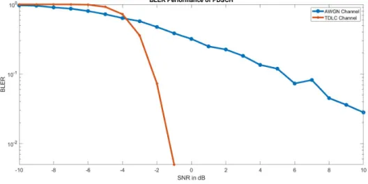
The channel estimator used for PDSCH is least square, followed by tone averaging and linear interpolation in time. The block error rate performance is highly dependent on the channel quality between the base station and the receiver. It delivers comprehensive performance and improved mobile broadband experience in terms of data rates with the help of transmission using OFDM (Orthogonal Frequency Division Multiplexing).
Transmission Scheme & Bandwidth parts
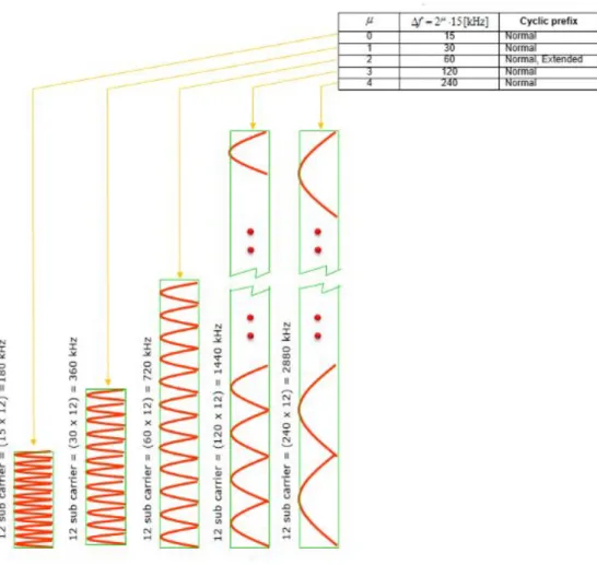
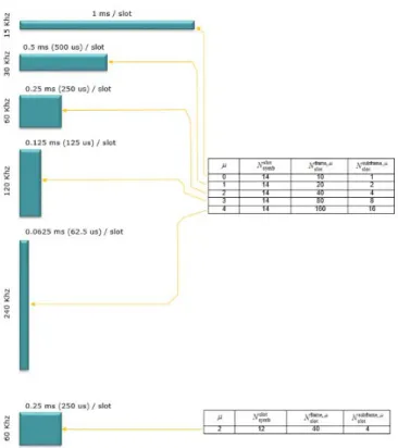
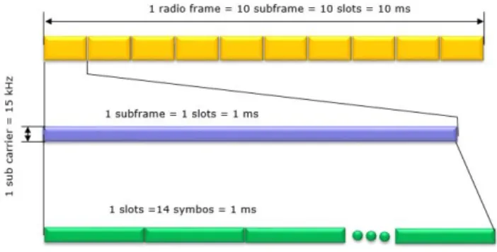
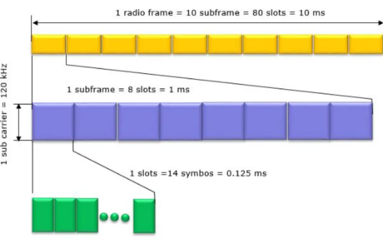
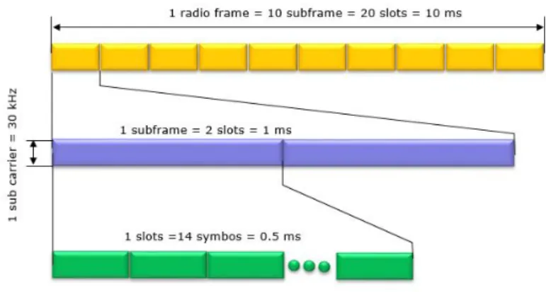
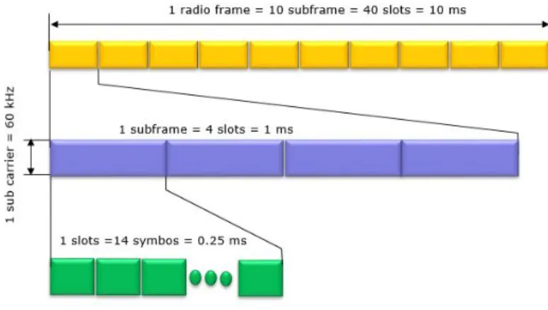
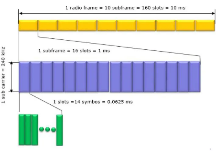
Numerologies & Frame Structure
Duplex Mode in 5G
- Time Division Duplexing (TDD)
- Frequency Division Duplex (FDD)
- Half Duplex FDD
- The Physical Downlink Shared Channel
- The Physical Broadcast Channel
- The Physical Downlink Control Channel
- The Physical Uplink shared Channel
- The Physical Random-Access Channel
The physical layer is responsible for modulation, multiple antenna processing, coding and mapping the signal to the appropriate time-frequency source. Physical channel to transport channel mapping is also handled by it. This corresponds to the aggregation of time frequency resources used for the transmission of the given transport channel, which is associated with their physical channels.
Within each TTI, one or two transport blocks of variable size arrive at the physical layer and are transmitted over the radio interface. Rate matching which helps to match the number of coded bits to the total number of the scheduled resource. After the mapping we go for IFFT and CP insertion at each of the transmitter antennas of the downlink.
This carries the bulk of the information needed to access the network. PBCH carries system information for UEs. From the name, it is clear that the functionality of this channel is to provide scheduling decisions necessary for reception of the PDSCH and also schedule grants that enable transmission on the PUSCH.
- Demodulation Reference Signals
- Phase Tracking reference Signals
- Channel State Information reference Signals
- Tracking Reference signals
- Sounding Reference Signal
Unlike the PUCCH in LTE where it is located at the cell edges with fixed timing and duration in NR, we have flexibility to do this. The PUCCH is designed based on 5 formats: PUCCH formats 0,2 which use 1 or 2 OFDM symbols in time the PUCCH formats 1,3,4 can use 4 to 14 OFDM symbols. The main purpose of PRACH is to achieve the synchronization between gNB and the UE (user equipment).
The receiver needs the DCI carried on the PDCCH to decode the PDSCH data. After that, the data transmitted on the PDCCH is decoded at the receiver which provides the DCI the receiver needs to decode the actual data. Here is a brief overview of the flow of the PDSCH transmitter and receiver chain[2].
PDSCH Transmitter
- Transport block Generation and CRC attachment
- LDPC base Graph Selection
- Code Block Segmentation and CRC attachment
- LDPC coding and Rate Matching
- Code Block Concatenation
- Scrambling and Modulation
- Mapping to Physical Resources
- IFFT and CP Insertion
After LDPC encoding, we re-add the padding bits that we discarded during data processing for LDPC encoding. Rate matching is done to ensure we are sending the correct data and not sending duplicate data. Bit Selection: This is done by writing the LDPC encoded data into a circular buffer and then reading the data according to the redundancy version.
Bit Interleaving: After bit selection, the data is written in rows, where the number of rows is determined by the modulation order used in NR. Then the data is read column-wise, that is, the first element of each row is read, followed by the second element of other rows. In this block, the data from each of the rate-matched blocks is concatenated in a serial fashion.
After the LDPC encryption is completed, there is no point in keeping the data in its previous form and so concatenation follows. The purpose of this block is to randomize interference, allowing the decoder to decode the data effectively, since the received signal strength from two adjacent base stations may be approximately equal.
Channel Models
The need to use 4096 FFT points instead of 2048 or less is that the PDSCH data, when configured for a portion of the total bandwidth of 275 resource blocks, has a total of 3300 subcarriers. NR specifies two different CP 320 lengths for the first and 8th. symbol in the slot, and for the rest of the symbol its length is 288.
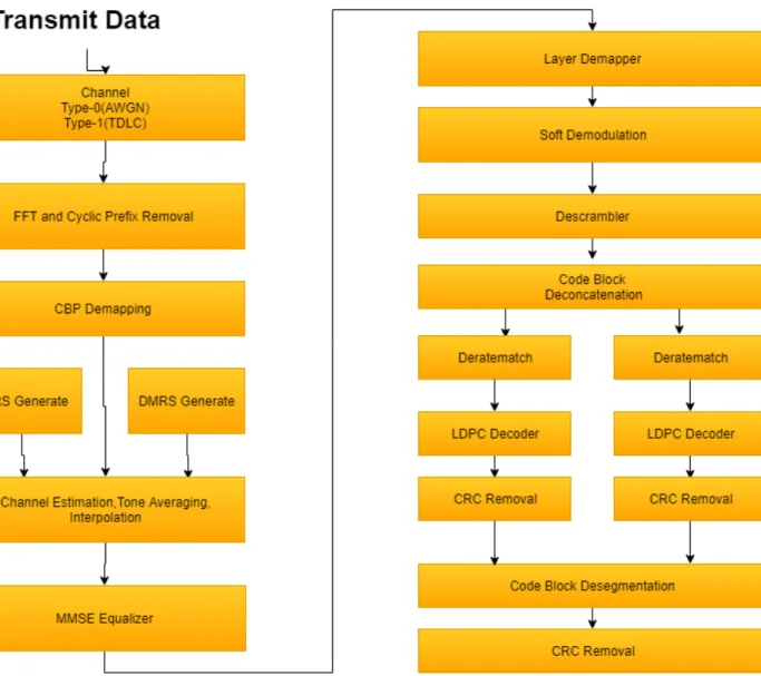
PDSCH Receiver
- FFT and CP Removal
- Resource Demapping
- DMRS and PTRS Generation
- Channel Estimation,Tone averaging and Interpolation
- MMSE Equalizer
- Layer De-Mapping
- Soft Demodulation, Descrambling, Codeblock De-Concatenation
- LDPC Decoding and De-rate matching
- Code Block Desegmentation and CRC Removal
No, as mentioned earlier, there is a mapping between the layer map and the antenna map block, so the output of the layer unmapping block and the antenna unmapping block is the same[2]. The receiver knows well in hand what the configuration type is, map type, single or dual DMRS symbol, etc. After evaluating the channel in the RE where the DMRS is placed, we move on to the average tone.
The interpolation is performed as follows: Up to the first DMRS symbol, the channel estimates for the first DMSR symbols are repeated. After the last DMRS symbol and until the last symbol, we simply repeat the channel estimates for the last DMRS symbol. After the data has been equalized by the MMSE equalizer, it passes through layer-de-mapper, which is the counterpart of layer-mapper.
The LDPC decoding block is followed by de-rate matching, which is the inverse of rate matching. After this, we plot the block error rate performance for the transmitted data with respect to increasing snrdB, which is shown in the next section.
PDSCH Results and Simulation Parameters
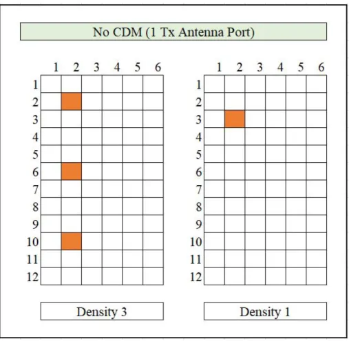
Whenever a CSI-RS is configured, it can be used by different devices to estimate their channel, provided that the corresponding device is configured accordingly. The point to be noted is that CSI-RS multiplexed in the time/frequency domain does not necessarily need to complement the adjacent subcarrier/OFDM symbol respectively. Moreover, if we look at the CSI-RS frequency, then we can notice that CSI-RS can have a density equal to 1 in which case it will be transmitted in every resource block for the full bandwidth.
But CSI-RS can also be transmitted with a density of 1/2, in which case it will be transmitted in the alternate resource block. The CSI-RS configuration in such a case will indicate that we are transmitting in even or odd-numbered resource blocks. If the single port CSI-RS is configured with density more than 1, then the number of CSI resources per resource block be equal to the density.
Periodic: In this case, the CSI-RS transmission is assumed to be configured to occur every Sig Mth time slot, where M ranges from 4 to 640. Aperiodic: In this case, there is no periodicity in CSI-RS transmission, but a device can be configured by signaling in DCI.
Zero power or Muted CSI RS
Semi-persistent: In this case, everything corresponds to periodic configuration, the only difference is that the activation and deactivation of CSI-RS transmission is controlled by the MAC. Specifically, Zero-power does not mean that there is no transmission in the resource element, but it means that the REs related to the ZP CSI-RS are used for NZP-CSI RS transmission for the other device.
CSI-Interference Measurement
CSI Generation
CSI Mapping to Physical Resource
The CSI reports consist of three parameters RI (Rank Indicator), PMI (Precoding Matrix Index) and CQI (Channel Quality Information), which are fed back to the transmitter. However, this report is the advice to the broadcaster about the channel, but the broadcaster is free to decide whether to follow that advice or not. In the event that the sender does not follow the UE's recommendation, this must be signaled to the UE in some way.
It is a recommendation sent by the UE to the base station about how many independent layers can be transmitted by the base station. It says which precoding matrix should be used by the transmitter for beamforming when operating in the spatial multiplexing mode. The precoding matrix index belongs to the set of indices corresponding to a particular matrix from the codebook.
This includes the highest modulation and coding scheme to be used by the transmitter. Usually, for MCS the notion is to return the index for which the coded block error rate is less than 10 percent.
Types of Channel State Reports
The point to note here is that the rate should not increase the maximum channel capacity limit as specified by Shannon. The rank indicator is not sent very often, assuming that the appropriate rank varies relatively more slowly than the channel conditions for PMI and RI. Aperiodic reports, on the other hand, are more detailed and are only sent when triggered exclusively by the base station. It is sent on PUSCH which is capable of carrying more amount of data.
The overhead in terms of bits is not a major problem here, as it is reasonable to assume that the base station will transmit a larger number of bits and therefore be requested exclusively for the aperiodic report. Broadband reports: This means that the recommendation sent by the UE is valid over the entire bandwidth. UE Configured Reports: This report means that the report has been generated by the UE for a few specific subbands and the report is only valid for that bandwidth.
According to the data, the channel model used for the simulation was both AWGN and TDLC as defined in the specifications for 5G-NR.
Basics of precoding
System Model
Generation of CSI-RS
Channel Estimator
RI and PMI estimation algorithm
After calculating this, we plug into the channel capacity equation and sum it over all possible layers. Having the channel state information increases the performance of manifolds and the base station uses the precoding weights to beamform in the direction of a specific UE when operating in spatial multiplexing mode. Moreover, the modulation order and coding scheme used and the number of independent layers for transmission also depend on the downlink channel quality.
The channel estimates are used for Post MMSE SINR calculation per subcarrier for a given rank and the precoding matrix indices. The PMMSE SINR is used to find the channel capacity per subcarrier. The ranking and the precoding matrix indices that maximize the channel capacity are fed back to the gNB. The MCS calculation is done by mapping the SINR with the MCS specified in such a way that the block error rate is less than 10 percent and also keeping in mind that the rate should not increase the capacity for AWGN, ie Log2(1+SNR ). Due to the scarcity of time, I could not calculate and validate the PMI, RI and CQI algorithms.
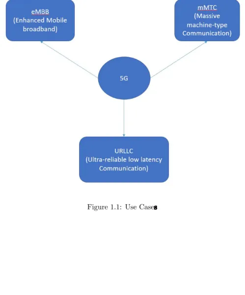
Use Cases
Bandwidth occupied by a resource grid in various numerologies
Time duration of Slots in various numerologies
Frame Structure for Numerology 0
Frame Structure for Numerology 1
Frame Structure for Numerology 2
Frame Structure for Numerology 3
Frame Structure for Numerology 4
Block Diagram of PDSCH transmitter
Block Diagram of PDSCH Receiver
Block Error Rate Performance Of PDSCH
Simulation Parameters
CSI Mapping for 1 Antenna Port Configured
CSI Mapping for 4 Antenna Port2CDM × 2F DM Configured
CSI Mapping for 4 Antenna Port 2CDM × 2T DM Configured
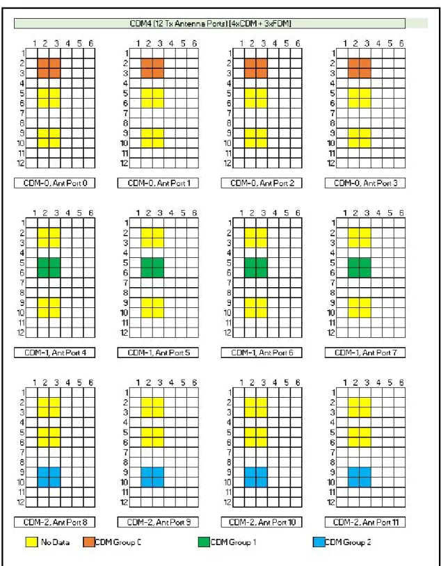
CSI Mapping for 12 Antenna Port Configured
CSI Mapping for 32 Antenna Port Configured
CSI RS location within a slot
Mean Square Error for 8-port Configured
Mean Square Error for 32-port Configured