Furthermore, designing the WPT system involves numerous geometric modifications to the 3-D FEA model. The change in mutual inductance affects the power transfer capability and efficiency of the entire system.
Introduction
Literature Review
Numerical Method
- Finite Difference Method (FDM)
- Finite Element Analysis (FEA)
- The Moment Method (MoM)
The most promising used numerical methods include the finite difference method (FDM), finite element analysis (FEA) and method of moments (MoM). The finite difference method is one of the oldest numerical methods used to solve the magnetic problem.
Analytical Method
- Biot Savert Law
- Magnetic Equivalent Circuit (MEC)
- Harmonic Method (HM)
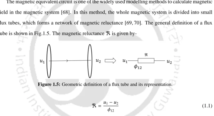
But the magnetic problem involving multiple boundaries, the imaging method is not suitable [67]. The equivalent magnetic circuit is one of the widely used modeling methods for calculating the magnetic field in the magnetic system [68].
Research Motivation
Then, Poisson's or Laplace's equation is solved in each region using the separation of variables method. The characteristics of different magnetic field modeling techniques are presented in 1.1 Table 1.1: Comparison of magnetic field modeling techniques.
Aim of the thesis
Thesis Contribution
Thesis Overview
This computational power increases further as the dimensions of the coil system increase [80]. Therefore, the analytical model is more suitable in the initial design and optimization of the winding system.
Analytical Model
- System Description and Assumptions
- Solution of the magnetic vector potential and scalar potential
- Magnetic vector potential in coil
- Solution of magnetic scalar potential in air medium
- Modelling of the current density distribution
- Boundary conditions
Using (2.1) and (2.6), the magnetic field density B can be written in terms of current density as. To calculate the magnetic field density using (2.6), the coefficients of the potentials for each region must be known.
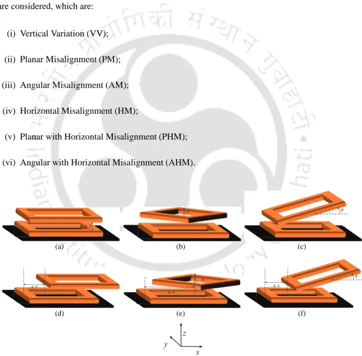
Possible Misalignments
Mutual Inductance Calculation
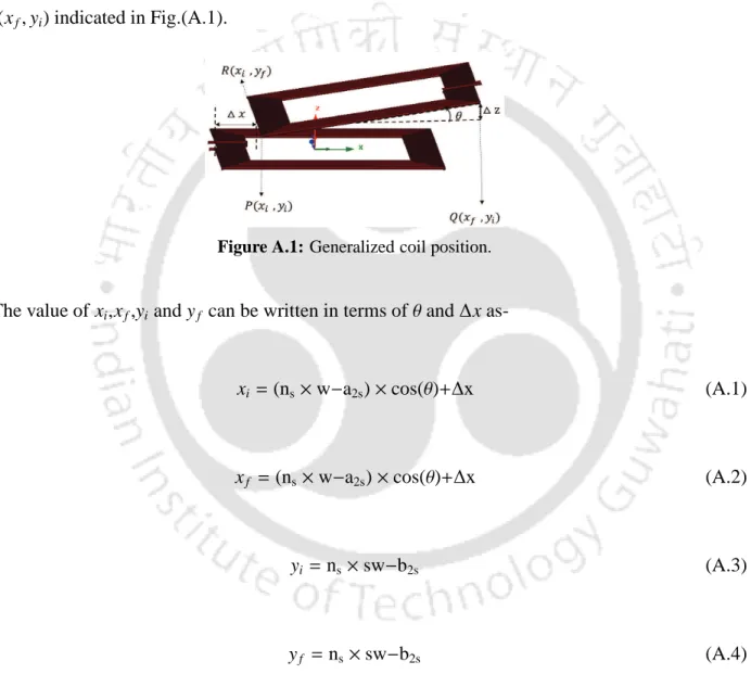
3-D Analytical Model for Calculation of Mutual Inductance for Different Mismatches in Wireless Power Transfer System. Here, the expressions contain the distortion parameters such as ∆z, θ, ∆x, and α, due to the dependence of the surface integration limit on the distortion parameters (the detailed derivation is given in Appendix A. However, for VV and HM, both (2.44 ) and (2.45) can be used to determine the mutual inductance by setting θandα equal to zero.
Verification of Analytical Model
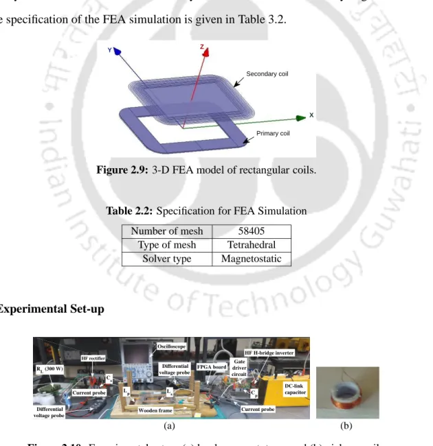
- FEA Simulation
- Experimental Set-up
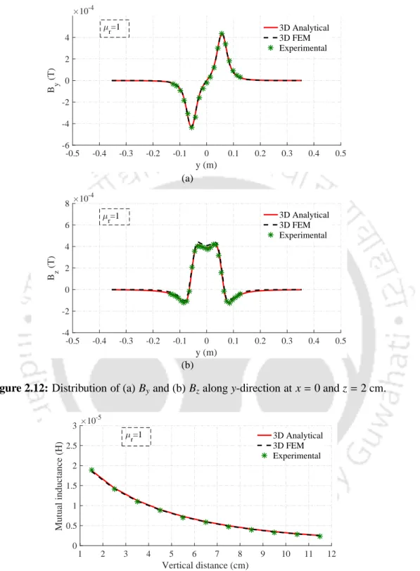
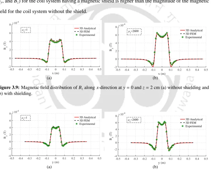
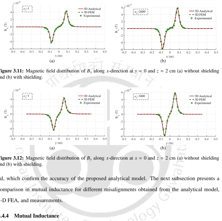
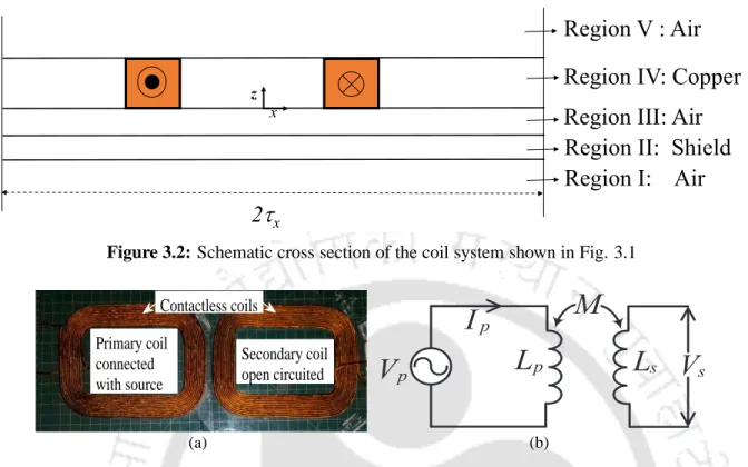
- Magnetic Field Distribution in the Air Gap
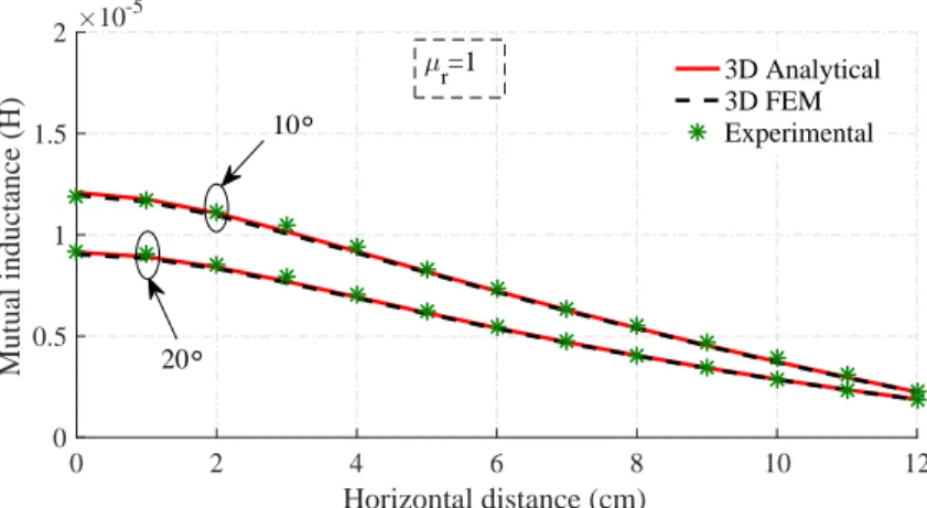
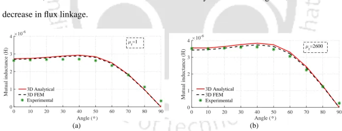
- Mutual Inductance
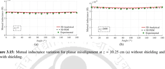
The next sub-section compares the mutual inductance obtained from the analytical model with the measurement and FEA results. The proposed analytical model is used to calculate the mutual inductance for different mismatches. The change in mutual inductance for the case when the secondary coil moves along the x direction is reported in Fig.
Summary
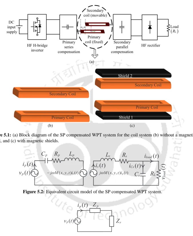
3-D analytical model for calculation of mutual inductance for various shielding mismatches in a WPT system. The previous chapter presented a 3-D analytical model to calculate the mutual inductance for an air-core coil system without a magnetic shield for a WPT system. In this chapter, a 3-D analytical model is presented to calculate the mutual inductance and magnetic flux density distribution in an air medium for a coil system incorporating magnetic shielding with finite permeability.
Analytical modelling
Coil System Overview
The base of the primary coil (region III) with relative permeability one (µr = 1) is considered as air medium, and region IV is a primary coil carrying source current. The magnetic vector potential is used in the region where the current source is present, and magnetic scalar potentials are used in other regions [94]. To calculate the magnetic field in the assigned areas, the magnetic potential in each area must be known.
Magnetic Field Description
- Region IV
- Region I, II, III, and V
The solution of the magnetic vector potential is given by considering Poisson's and Laplace's equations. The unknown coefficients involved in the magnetic vector potential given in (3.6) depend on the boundary conditions. Here, the magnetic vector potential for the current-flowing region (primary coil) is revealed.
Boundary Conditions
The scalar potentials used here are different compared to the magnetic scalar potential used in Chapter 2 due to different boundary conditions. This subsection defined magnetic vector and scalar potential with unknown coefficients for each assigned region. After calculating unknown coefficients for the magnetic potentials, the magnetic potentials (3.6) and (3.10) can be used to calculate the self-inductance and mutual inductances for different misalignments, respectively.
Possible Misalignments
Depending on the different displacements of the secondary coil relative to the primary coil, discrepancies are taken into account. Compared to the coil system discussed in Chapter 2, the only difference is that in Chapter 2 the primary coil is surrounded by air, while here there is a magnetic shield near the primary coil. Therefore, the same mismatches are taken into account, which are:. v) Planar with horizontal displacement (PHM);. vi) Angles with horizontal deflection (AHM).
Verification of Analytical Model
- FEA Simulation
- Experimental Set-up
- Magnetic Field Distribution in the Air Gap
- Mutual Inductance
- Comparison with method given in [1]
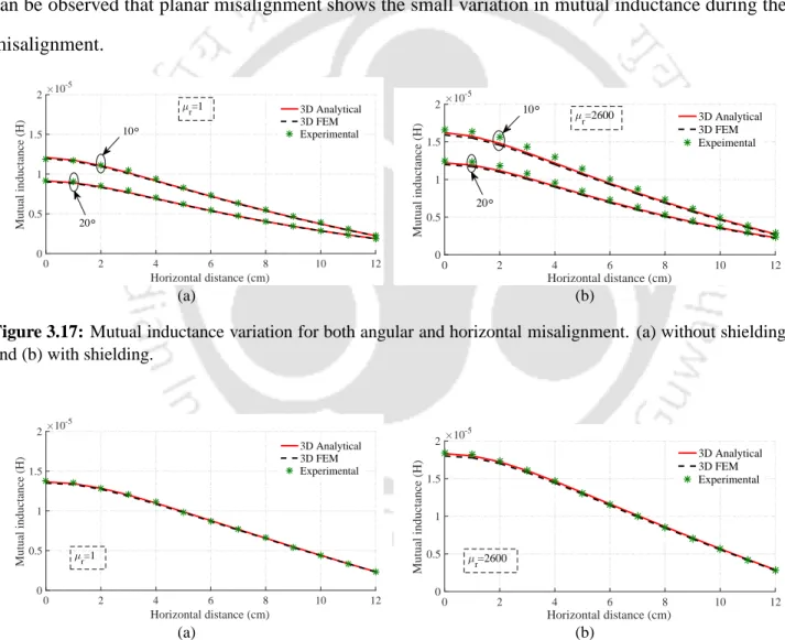
Here, mutual inductance decreases as the secondary coil moves along the z-axis due to the decrease in flux coupling. The variation in mutual inductance for the case where the secondary coil moves along the x-direction is shown in Fig. In this subsection, the variation in mutual inductance for different misalignments is shown in Fig.
Summary
System Overview
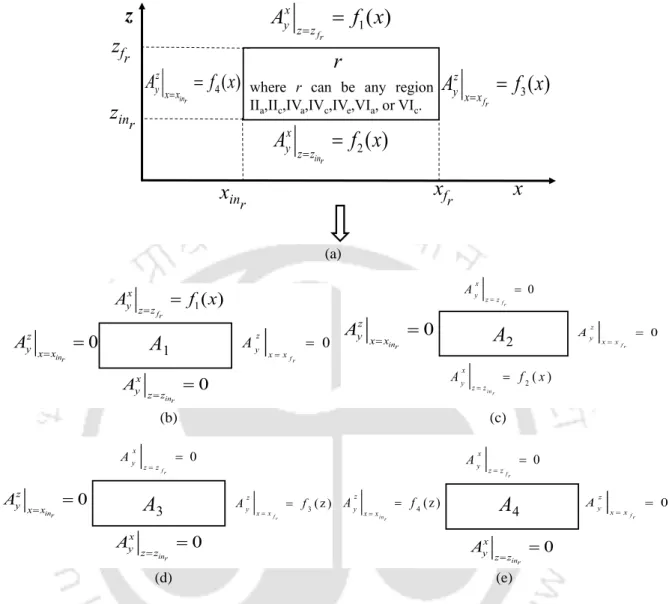
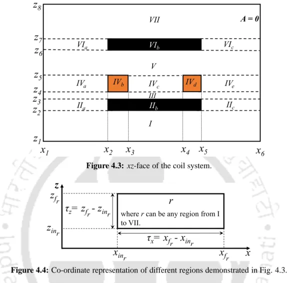
Areas IVa and IVe represent the air medium to the left and right of the primary TH. Region IVc represents the air medium between the two sides of the coil of the primary coil. Region r may be any of regions I to V II as shown in FIG.
Magnetic Field Description
A region r has been defined to represent the magnetic vector potential for each subdomain, as shown in Fig. The magnetic field for each described region is calculated by magnetic vector potential, which is obtained using the Poisson and Laplace equations, as discussed in the next subsection. The next subsection presents expressions for vector potentials for each region discussed in Section 4.2.1.
Magnetic Vector Potentials
- Regions II b , IV b , IV d , and V I b
- Regions III and V
- Regions II a , II c , IV a , IV c , IV e , V I a , and V I c
- Regions I and V II
The magnetic vector potential on three sides of these regions is zero, making the interface condition applicable only on one side for this region. The expression of the magnetic vector potential for regions I and V II is obtained by using cr =0 and dr =0 in (4.14), respectively. To calculate the magnetic field density using (4.3), the unknown coefficients of magnetic vector potentials should be known for each region.
Boundary Conditions
The accuracy and computational time of the subdomain model depends on the maximum number of harmonics considered in the solution. Further, the magnetic field analytical results are compared with the 2-D FEA results in the next subsection. In this case, the distribution of the magnetic field is symmetrical about the center of the coil.
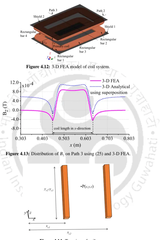
Superposition of Two 2-D Subdomain Models
A Subdomain Analytical Model of a Coil System with Magnetic Shields of Finite Dimensions and Finite Permeability for WPT Systems. Since fxz(x,y,z) varies with the y direction, as shown in Figure 4.16(b), multiplying it by the 2-D subdomain model (xz plane) facilitates the calculation of the magnetic field in the third ( y-) direction. A Subdomain Analytical Model of a Coil System with Magnetic Shields of Finite Dimensions and Finite Permeability for WPT Systems.
Verification of Analytical Model
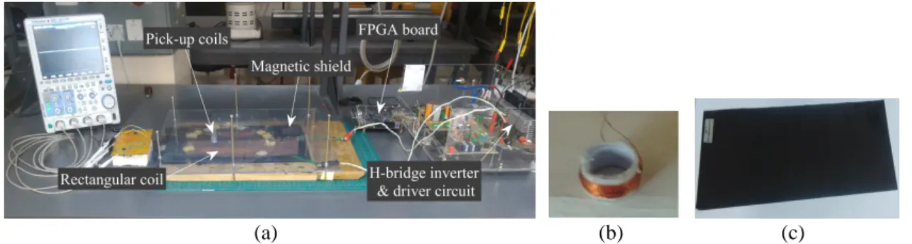
Experimental Setup
The magnetic field distributions obtained from (4.63) and 3-D FEA are compared with measurements in the next section. Cyclone-II FPGA board is used to generate the pulses to drive the MOSFETs (IRFP450) of the H-bridge inverter.
Results Description
4.24(a) and (b), it is observed that as misalignment increases, the value of mutual inductance decreases due to decrease in the flux coupling in the secondary coil. 4.24(c), it can be seen that as the separation between the primary and secondary coil arrangements increases, the value of mutual inductance decreases due to decrease in the magnitude of the magnetic field density.
Summary
The impact of change in the mutual inductance on system parameters was presented in [102-. In this chapter, an analytical model was presented to predict the variation in the electrical parameter of the SP-compensated WPT system during misalignments. For determining the variation in the electrical parameter of the SP-compensated WPT system, the mutual inductance for different misalignments was used as direct input to the steady-state model.
System Description and Mathematical Model
System Description
Steady-State Model
- Modelling of the Primary Side
- Modelling of the Secondary Side
The total impedance Zt of the SP-compensated WPT system (Fig. 5.3), as seen through the source, is given by. The instantaneous input power of the compensated primary coil pp(t) and the active power PP are calculated using (5.16) and (5.17), respectively. The instantaneous power of the load pload(t) and the active power Pload on the secondary side are obtained by (5.29) and (5.30), respectively.
Experimental Setup Description
C′p Primary side compensation capacitor for winding system having magnetic shield at M=35µH 31.33 nF C′s Secondary side compensation capacitor for winding system with magnetic shield 13.87 nF.
Results and Discussion
Results with Different Misalignments
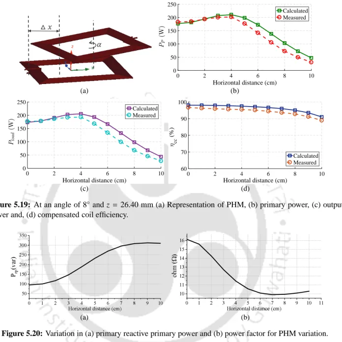
Here it can be seen that as the secondary coil moves away from the primary coil, the reactive power increases while the power factor decreases. Here it is observed that during this misalignment, the reactive power and power factor remain constant. As the misalignment between the primary and secondary coil increases, the reactive power of the primary coil increases, while the power factor decreases.
Variation in electrical parameter for coil system having magnetic shields
From the above discussion, it is concluded that VV shows the largest deviation in electrical parameters among all six mismatches.
Summary
This model can be used to analyze the component voltage of the SP compensated WPT system. Therefore, the proposed method can be adopted in the initial design process of the SP-compensated WPT system. The results of the analytical model are compared with the 3-D FEA model and the measurements, and a good agreement is found.
Limitations of the Work
The mutual inductance of the 3-D subdomain model was compared with FEA results and measurement. The proposed subdomain model facilitates changing the parameters (length, width and permeability) of magnetic shields. The results of the proposed subdomain model are acceptably accurate for initial design and optimization of the WPT system with magnetic shielding of finite dimension and permeability.
Scope for Future Research
In this section the boundary condition between each region of the winding system shown in Fig.
Regions with Applied Boundary Conditions
Magnetic Vector Potential of Different Regions
General Solution of Magnetic Vector Potential
The magnetic vector potential of the regions of the coil system is governed by the Laplace equation given in (B.47). Solving (B.47) using the method of separation of variables, the solution Ay in Cartesian coordinates (x,z) can be written as
Derivation of magnetic vector potential according to imposed boundary con-
- Block diagram of inductively coupled WPT system
- Classification of available methods to model a coil system
- Division of magnetic problem into grid points
- Division of magnetic problem into different mesh
- Geometric definition of a flux tube and its representation
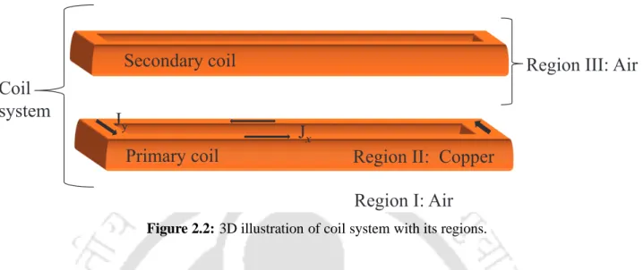
- Classification of available methods to model coil system shown in Fig. 2.2
- Arrangement of coils
- The actual coil and its approximation
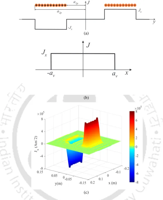
- Current density distribution of J x (a) along y-direction, (b) along x-direction, and (c)
- xz face of rectangular coil
- Schematic of studied variations (a) vertical variation (VV), (b) planar misalignment
- Experimental set-up (a) hardware prototype, and (b) pick-up coil
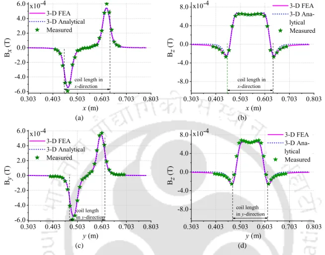
- Distribution of (a) B x and (b) B z along x-direction at y = 0 and z = 2 cm
- Distribution of (a) B y and (b) B z along y-direction at x = 0 and z = 2 cm
- Mutual inductance variation in z-direction without shielding
- Mutual inductance variation for angular misalignment
- Mutual inductance variation for planar misalignment at z = 10.25 cm
- Mutual inductance variation for horizontal misalignment at z = 1.35 cm
- Mutual inductance variation for both angular and horizontal misalignment
- Mutual inductance variation for both planar and horizontal misalignment
- Schematic cross section of the coil system shown in Fig. 3.1
- WPT system having (a) an actual coils, and (b) equivalent circuit model of contactless
- xz face of rectangular coil
- Schematic of studied variations (a) vertical variation (VV), (b) planar misalignment,
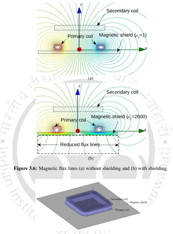
- Magnetic flux lines (a) without shielding and (b) with shielding
- Experimental set-up (a) hardware prototype, (b) pick-up coil and (c) magnetic shield. 56
Li, “Experimental study on asymmetric wireless power transmission system for electric vehicles considering iron chassis,” IEEE Trans. Rome, “Modern Advances in Wireless Power Transfer Systems for Road Powered Electric Vehicles,” IEEE Trans. Mi, “Inductive and capacitive combined wireless power transmission system with lc-compensated topology,” IEEE Trans.