Optimal Strain Gage Locations for Experimental Determination of Stress Intensity Factors

Among all experimental techniques, strain measurement techniques are relatively inexpensive, simple, and easy to use for determining SIFs. Further, a modified strain measurement technique for the experimental determination of mixed-mode SIFs is also proposed in the present investigation.

4.14 Graph of ln(  aa ) versus ln( ) r showing variation of the r max with the Poisson’s ratio 

Introduction

Introduction to fracture mechanics
Importance of fracture mechanics approach to design
Methods of analysis: Linear elastic fracture mechanics
Elastic plastic fracture mechanics
Fracture mechanics parameters

Strain energy release rate
Stress intensity factor
J- integral
Crack opening displacement

Stress intensity factors for different modes of loading
Methods for the determination of stress intensity factors

Analytical methods
Numerical methods
Experimental methods

Principle of operation of the electrical resistance strain gage
Bonded metallic foil strain gages
Motivation
Organization of the thesis

Displacements of the crack surface occur in the plane of the crack and parallel to the leading edge of the crack. Strain gauges are attached to the body surface and are part of it.

Literature Review

Strain gage techniques for determination of mode I SIF
Strain gage techniques for determination of mode II SIFs
Strain gage techniques for determination of mixed mode I/II SIFs
Summary of literature review and objectives

Dally and Sanford [28] proposed a strain gauge technique to determine the dynamic SIF of mode I of a propagating crack. Marur and Tippur [46] developed a strain gauge technique for determining complex SIF in bimaterial systems.

Theoretical Background and Formulations

The generalized Westergaard approach

Leading terms for mode I loading
Leading terms for mode II loading

Using Cauchy-Riemann equations and air stress function approximation, the stress components for mode I in the absence of body forces can be given as. and the stress components for the mode II can be obtained as. The displacement field near the crack tip under plane stress conditions can be obtained as.

Figure 3.1 The complex plane at the crack tip

Thus by placing a single strain gauge (Fig. 3.4 ) on the radial line OS defined by  (Eq. 3.27)) at a suitable radial distance r from the crack tip and orienting the gauge at an angle  (according to Eq. It can be seen from equations 3.26) and (3.27) that KI can also be determined by placing a strain gauge on line OT which makes an angle of - with respect to the crack axis. Thus, these are the radial lines on each of which a strain gauge must be attached according to the DS technique, for the determination of KI.

Figure 3.2 Different zones at the crack tip [22]

Rmax can therefore conversely be defined as the extent of validity of Eq. 3.28) or the extension of the three parameter representations along the radial line defined by  (Eq. To take full advantage of the DS technique for avoiding strain gradient, plasticity and 3D effects, Eq. 3.32) shows that the strain gauge can be climbed very near rmax (but not beyond rmax) however the meter readings can be expected to obey Eq. Thus the experimentalist can easily establish valid gauge locations using Eq. 3.29) depending on the material of the specimen.

Figure 3.5 (a) Plot of ln(  aa ) versus ln( ) r (b) linear and non-linear variation of ln(  aa ) and ln( ) r

Since for negative value of , the angle  is also negative, the strain component bb defined by - and - as shown in fig. Thus, if the strain gages are pasted along the positive gage line (line OP) along the  direction and along the negative gage line (line OQ) along the  direction, then the measured strains would be in accordance with Eq. provided the gauges are located within Zone II or the extent of applicability of these equations. 3.40) is added and multiplied by r. It also appears from Eq. 3.45) and (3.46), that at least two strain gauges each at an angle of  with the crack axis must be placed along the positive and negative gage lines (as shown in Fig. 3.7) for the determination of KI and KII.

Figure 3.6 Strain gage location and orientation for mixed mode

Proposed modified Dally and Berger technique

It should be noted that the radial distance from the crack tip to the corresponding strain gauges on the positive and negative gauge lines must be the same (Fig. 3.9) for the calculation of the LHS quantities of Eqs. It is clear that all strain gauges should be located within the dominant zone of the above-mentioned coefficients, i.e. zone II, and at the same time should not be placed very close to the crack tip. Therefore, prior knowledge of valid radial locations for strain gauges is essential for successful application of the modified Dally and Berger technique for the accurate determination of KI and KII.

Figure 3.9 Proposed gage locations for a mixed mode cracked body

Determination of maximum permissible radial location r max in mixed mode (I/II)

In order to account for Eqs. 3.53) and (3.54), the maximum allowed (or upper limit) radial location or range of validity of both equations. It should be noted that the radial distances from the crack tip to the corresponding points on the positive and negative gauge lines must be the same to calculate the LHS quantities from equations (3.61) and (3.62) and that the FEA meshes must be designed. accordingly. It is clear that the RHS quantities of Eqs. 3.53) and (3.54) can accurately represent LHS quantities (ie Eaa and Ebb obtained using FEA) up to a certain radial distance due to the small number of coefficients (or parameters) A A0, 2, B1, C C0, 1 and C2 are present in RHS amounts.

Finite element formulation

Eight nodded quadrilateral element
Quarter point elements (QPEs)
Collapsed six-nodded triangle quarter point elements

The singularity in the QPE is achieved by shifting the mid-side nodes on edges connected to the crack tip by a quarter of the length of the edge toward the crack tip. In the current study, the mid-side nodes of the selected Q8 element are shifted to quarter points to generate QPEs around the crack tip. The displacement u along the x-axis is given by. 3.96) and differentiate with respect to x, then the strain is in the x direction along the x axis. 3.97) shows that the strain singularity along the x-axis is 1.

Figure 3.10 Eight nodded quadrilateral isoparametric element represented in natural coordinates

Summary

Determination of r max for Mode I Cases

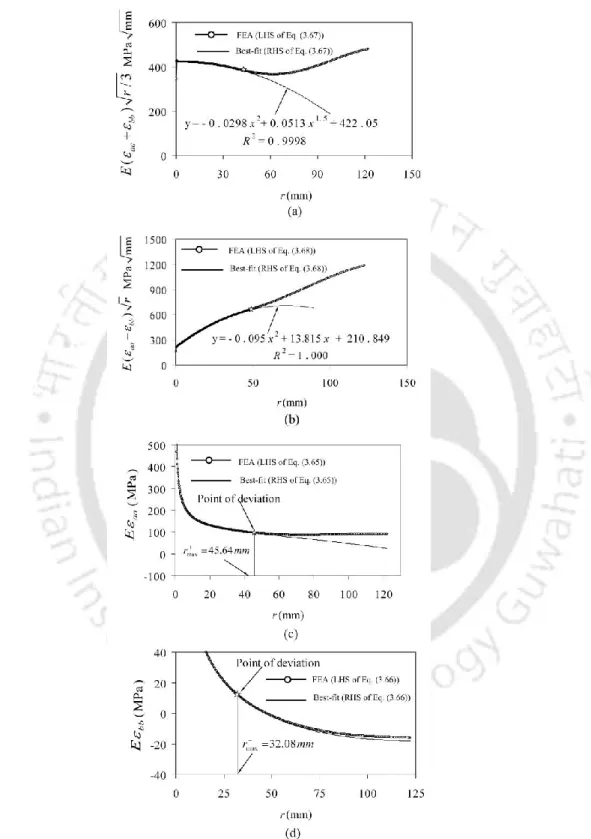
As explained in section 3.2, this measurement line starts at the crack tip and ends at the outer boundaries of the cracked plate. The deviation of this point from the straight line section may be due to the effect of the constant strain term (cf. These estimated values of rmax or the degree of validity of the three-parameter zone are marked in Fig.

Fig. 4.1(b). For evaluating the influence of the mesh refinement on r max values, three meshes of increasing mesh density for each of the plates with a b/  0.2 and 0.5 are considered for the convergence study as shown Figs

55] investigated the size of the singular term or singularity dominated zone (SDZ) of different cracked configurations. The decrease in the size of the SDZ with the increase of a b/ at higher values of a b/ was also observed by them. However, their work does not report an increase in the size of the SDZ with a b/.

Figure 4.7 Finite element meshes for the center cracked plate employed to study the effect of a b / on r max

The results of Table 4.4 clearly show that in the absence of boundary effects, crack length is the controlling parameter for changes in rmax. This implies that, in cases of small net ligament or higher a b/ values, the net ligament length (ba) is the controlling parameter for the change in rmax values. Initially, at low values of a b/ , the rmax value increases with increasing a b/ as the crack length is the controlling parameter due to the insignificance/absence of the boundary effect on rmax.

Fig. 4.11 shows the variation of ln    aa with ln   r on the gage line of the above configurations along with the point of deviation  ln  rmax  of the straight line portions

To further support this conclusion, we can observe in Table 4.5 approximately the same values of the ratio rmax/(b a ) for a b/ 0.5 and 0.7. The values of rmax/a corresponding to a b/ 0.2 and 0.3 are almost the same and significantly different from other values of a b/ , indicating the influence of the crack length, a. On the other hand, the values of rmax/(b a ) are almost the same for a b/ from 0.5 to 0.8, indicating the influence of boundary effects.

Determination of r max for edge cracked plates

In all the meshes, this line starts at the crack tip and ends at the outer boundaries of the cracked plate. The radial distances  r of each of the nodes on the gauge line from the crack tip are then calculated. Similar to the previous example, an explanation of this behavior of the rmax with a b/ is explored in the next section for edge-cracked plate.

Figure 4.15 (a) A typical edge cracked plate (b) solution domain for edge cracked plate Table 4.6 Geometric and material parameters of the edge cracked plate

Effect of the crack length and proximity of boundary on the r max

Conversely, the relative increase in the size of A0 tends to increase rmax, while the increase in the size of non-singular terms (relative to A0) decreases. 4.17, when a b/ increases, the magnitude of the singular term A0 has dominated over the magnitudes of the non-singular terms. Thus, the relative increase in the magnitude of A0 leads to an increase in the rmax value, while an increase in the magnitude of the non-singular terms results in a decrease in the value.

Figure 4.19 Variation of ln    aa with ln   r along the gage line for the edge cracked plates under plane stress condition with a b/ = 0.00625 to 0.05

Thus, aa along the entire measurement line for plane stress differs from the conditions of plane strain mainly due to the change in terms related to the material properties (E in. For a given geometry and boundary conditions, the increase in the size of the singular and non-singular terms with the increase of a b/ remain the same both for the state of plane stress and plane strain.The difference in the rmax values is therefore mainly due to the terms depending on the material properties, which assume different values in the conditions of plane stress and plane strain.

Figure 4.22 Comparison of plane stress and plane strain r max values for the edge cracked plate

Determination of r max for double edge cracked plates

In fact, this could be expected because as b/ increases, unlike previous examples, the crack tips in this configuration move away from their respective boundaries. This explanation is clearly based on the studies carried out on the effect of crack length and boundary proximity in the previous examples.

Figure 4.24(a) Typical mesh used for double edge cracked plate (b) enlarged view at the crack tip corresponding mesh

Eccentric center cracked plate subjected to uniform tensile stress

4.28(a) shows plots of ln aa versus ln r obtained using the values at the right crack tip for an eccentricity ratio of 15%. As the right crack tip is moved close to the boundary, the rmax values decrease due to the boundary effects as demonstrated in the previous sections. On the other hand, as the left crack tip moves away from the boundary, the rmax values obtained at this point increase as expected.

Figure 4.26 (a) Eccentric cracked plate; (b) solution domain for eccentric cracked plate Table 4.9 Geometric and material properties of eccentric center cracked plate

The strain gauge location at r4.88 mm by Dally and Sanford [22] could be considered very close to the crack tip compared to their corresponding rmax value. The strain measurements made at the gage locations used by Rizal and Homma [35] and Dally and Barker [33] would not be the same as predicted by Eq. 3.25) and therefore the measured SIF may be incorrect. 39] could be considered optimal or valid gage locations, and it can be expected that strain measurements will be close to the theoretical prediction given by Eq.

Table 4.11 Specimens and material properties used by various researchers

Summary

This chapter describes a general methodology for estimating the maximum allowable radial location for the accurate measurement of mixed-mode stress intensity factors (KI and KII), based on the theoretical formulations presented in Sections 3.5 and 3.6 for mixed-mode problems. This chapter also investigates the effectiveness of the proposed modified DB technique for the experimental determination of mixed-mode SIF, in which the calculated maximum allowable radial location is used to locate the optimal gauge locations. In this chapter, the influence of the ratio between the length and width of the crack and the state of stress on the optimal locations of strain measurements was also investigated.

Problem Definition

Accuracy of the proposed method in determining coefficients of stretch range expansion is substantiated and presented in this chapter by comparing the results of the present method with those of Xiao and Karihaloo [57]. 5.1(b) shows a typical FE mesh together with the enlarged view at the crack tip mesh (Fig. 5.1(c)) which ensures that the successive nodes from the crack tip on both the measurement lines are the same radial distance from the crack tip.

Determination of the r max for slant edge cracked plate

Thus, as expected, these ranges (i.e. rmax and rmax ) are different for the positive and negative measurement lines. In a similar way, the deviation point rmaks for the negative measurement line is obtained as in Fig. Showed. Since the rmaks and rmaks are different for positive and negative gauge lines, therefore the radial distance corresponding to the deviation points in Fig. .

Table 5.1 Geometric and material parameters of the numerical examples of the present work

Validation of the present approach for determination of coefficients

However, a significant difference can be noted in values of the coefficients A B C2, 1, 1 and C2 obtained using the present approach and those reported by Xiao and Karihaloo [57]. 5.11(a) shows comparison of Eaa values obtained by FEA, RHS of Eq. 3.65) with the coefficients reported by Xiao and Karihaloo [57] and RHS of Eq. 3.65) by substituting the coefficients obtained from the present approximation along the entire positive gauge line. A large error in predicted values by the coefficients of Xiao and Karihaloo [57] can be noticed (Fig. 5.12) even at small radial distances from the crack tip.

Figure 5.10 (a) determination of A A 0 , 2 and B 1 using the best-fit linear regression (b) determination of C C 0 , 1 and C 2 using the best-fit linear regression

Numerical validation of modified DB technique

The solution corresponding to the plane stress conditions of the previous example in section 5.5 is considered in this example for the purpose of comparison with the result for plane strain conditions. As in the case of mode I problems, the observed difference between the plane stress and plane strain values of the rmax can be explained as follows. As mentioned in the previous example, a reason for bell-shaped trend is due to the variation of the coefficients A A B C C and C2 with a b/ and which remains the same for both the plane stress and plane strain conditions.

Figure 5.14 Results for determination of the r max for SECP with a b /  0.3 : (a) determination of

Summary

Thus, the difference in the rmax values is mainly due to the terms associated with Poisson's ratio. The present chapter describes experimental verification for determining optimal radial locations of strain gauges using the proposed procedures described in previous chapters for mode-I and mixed mode I/II loading conditions. Experiments have been conducted with mode I as well as mixed mode I/II loading and SIFs have been determined based on strain gage readings.

Description of the test specimen

Specimens of PMMA have been prepared to perform experiments corresponding to mode-I as well as mixed mode (I/II) loading conditions. In all experiments in the present study, the width b of the specimens is 150 mm and the thickness is 5.6 mm. Then, a sharp crack of length 1 mm for open state and length 1.5 mm for mixed state is introduced using a jeweler's saw with a thickness of 0.22 mm.

Figure 6.1 (a) A typical mode I specimen (b) mixed mode specimen

Experimental determination of material properties of PMMA

In the third case (Table 6.1) similar samples were used as in the second case but with larger dimensions. Analogous to the first case, here also Young's modulus and Poisson's ratio were measured from the slopes of these best-fit lines. Young's modulus and the Poisson's ratio were obtained from the best-fit lines in a similar way to those in the first and second cases.

Table 6.1 Details of test specimens for determination of E and  of PMMA Case Test Specimen

Experimental verification of optimal strain gage locations

Numerical evaluation of r max for mode I experimental specimen
Numerical evaluation of r max for mixed mode experimental specimen
Details of experiments
Experimental results for verification of optimal strain gage locations in mode I

Results for a/b = 0.293
Results for a/b = 0.493

6.22, all strain gauges have been pasted along the measurement line () and maintain the correct orientation. Based on these, strain gage locations have been decided in the present experiments for all the three configurations as shown in Table 6.7. It should be noted that similar trends have been obtained with the load data from other repeated tests, as the slopes of the best-fit straight lines in Figs.