Quantum Phases of Constrained Bosons in Low Dimensions

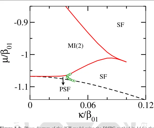
This is to certify that the thesis entitled "Quantum Phases of Constrained Bosons in Low Dimensions" submitted by me to the Indian Institute of Technology Guwahati, for the award of the degree of Ph.D., is a bona fide work done by me under the supervision of Dr. The regions marked with the green squares are enlarged in the insets, which show the signatures of the SF phase (top inset) and the PSF phase (bottom inset).

Quantum phase transitions

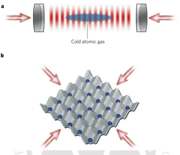
The ultracold atoms in optical lattices are an emerging quantum simulator that can overcome the shortcomings of conventional condensed matter systems. The first experimental observation of quantum phase transition in systems of ultracold atoms in a three-dimensional (3D) optical lattice was made by the group of I.

QPT in optical lattices

To circumvent this problem, several unique quantum simulators have been theoretically proposed and experimentally observed in recent years to mimic the QPTs in condensed matter systems. The unparalleled control over the system parameters using the sophisticated experimental techniques in such simulators has revealed a wealth of new physics in recent years.

Optical lattice

Ultracold bosons in optical lattice: The Bose-Hubbard model . 5

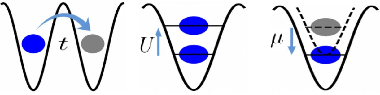
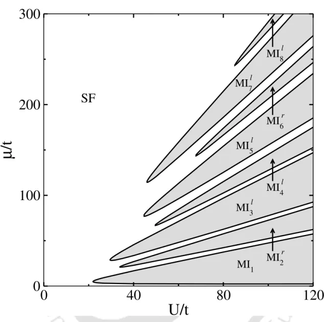
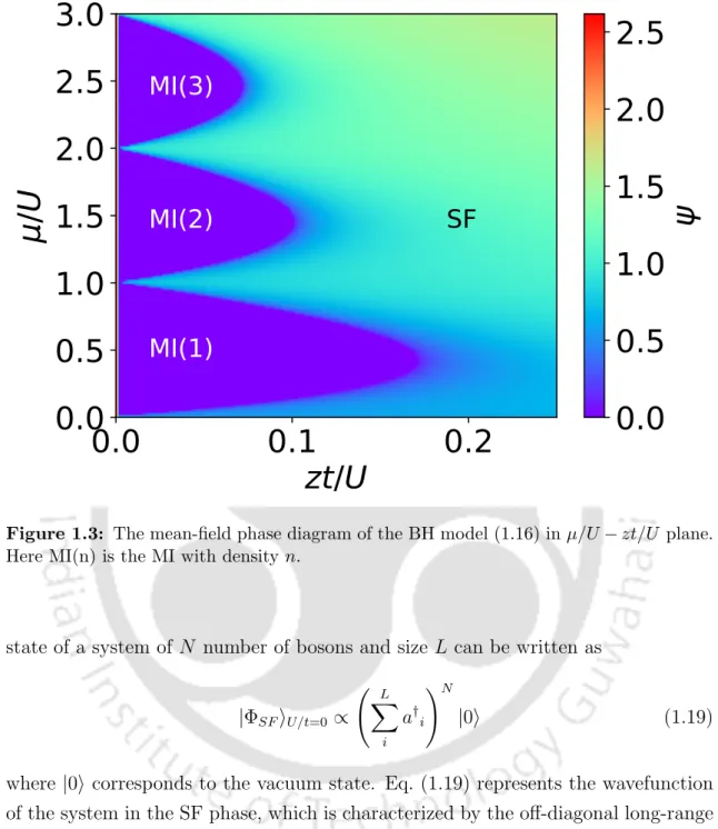
Below we briefly discuss the BH model and the SF-MI phase transition. However, in the weak interaction limit (or strong jumping), the system shows the SF phase (white region).

Figure 1.2: Figure depicts the significance of different parameters in the BH model given in Eq

QPT in superconducting circuits

Qubits

However, the quantum energy levels of a harmonic oscillator are uniformly spaced, making selective transition between two levels impossible. JJ can be used to construct qubits, which is an acronym for quantum bits, a device where we can achieve a selective transition between two levels.

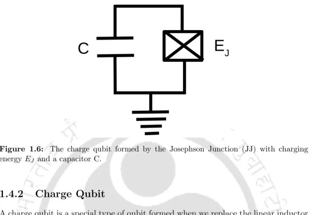
Charge Qubit

The presence of the gate electrode, which is connected to the qubits via coupling capacitors and operates at a fixed voltage, introduces some offset into the circuit. Since the evaluation of aν(q) turns out to be a tedious task, we rewrite the Hamiltonian in a more convenient way, in terms of a reduced charge basis |ni, as follows:.

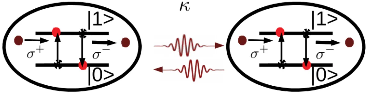
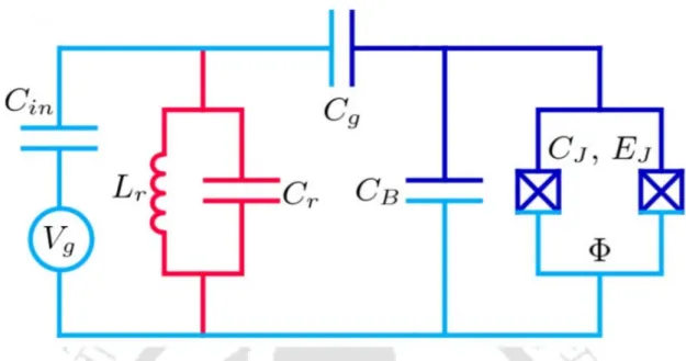
Circuit QED for transmons

Here we define a quantity that is the sum of the number of atoms and the number of photons in a single cavity, also known as the polariton number ni of the ith cavity, written as ni = σi+σ−i +b†ibi. The polariton number is a conserved quantity of the system as it commutes with the Hamiltonian given in Eq. Motivated by all the recent progress, in this thesis, we explore some of the interesting problems involving interacting bosons in low-dimensional lattices.

The primary focus of this thesis is to study the ground state properties of a particular many-particle system using various numerical methods.

Figure 1.7: Circuit diagram of a transmon qubit consisting of two JJs with capacitances C J and Josephson energy E J , a biasing capacitor C B and a gate capacitor C g connected to a resonator with capacitance C r and inductance L r

Chapterwise outline of the thesis

The ground state of the BH model is known to exhibit an SF-MI phase transition as a function of the t/U ratio, as already mentioned in Section 1. The ground state energy can be obtained as a function of the order parameter ψ by diagonalizing Eq. In the numerical approach, we use an iterative procedure to obtain a self-consistent value of the superfluid order parameter ψ to obtain the basic state of the system.

The MF theory for the BH model estimates the critical point for the SF-MI transition to be (U/zt)c ≈ 5.83.

Cluster Mean-field Theory (CMFT) approach

Exact Diagonalization (ED)

In principle, the ED method gives us a way to calculate the entire energy spectrum of the Hamiltonian representing a. If it is assumed that the maximum number of states per place is m, the dimension of the entire Hilbert space is D = mL, disregarding any symmetry in the system. This assumption enables us to write the Hamiltonian in a block diagonal form so that we can separately solve each block of the Hamiltonian.

Now if we further increase the value of p, we can improve the precision of the excited states.

Density matrix renormalization group (DMRG)

Finally we compare the different methods in the context of the phase diagram of the BH model in Fig. When the system size is L = l+ 2 +l0, the system block is increased at the expense of the environment block. Follow step 3-7 of the infinite DMRG algorithm until you reach the right edge kul0 = 1.

Now start growing the environment block at the expense of the system block until you reach where = 1 on the left.

Figure 3.1: (a)Illustration of a bilayer superlattice having periodicity equal to two show- show-ing the intra-layer and inter-layer interactions

Method

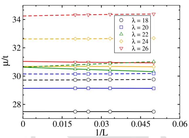
By recording the values ​​of UA,UB (in the case of TBCs) and UAB, we calculate the complete phase diagram in µ/tvs. We also consider some specific values ​​of lambda and vary the interactions to obtain the phase diagram as done in Ref. In our DMRG calculation, we assume system sizes of up to 100 sites and a binding dimension of 500.

Figure 3.2: The CMFT phase diagram when bosons in layer-A are softcore and in layer-B are HCBs

Results and Discussion

Hardcore constraint for bosons in layer-B

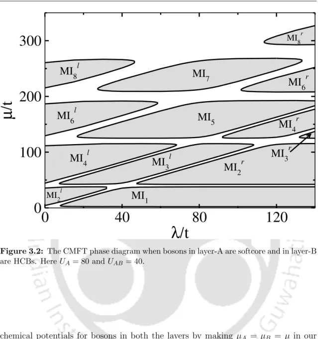
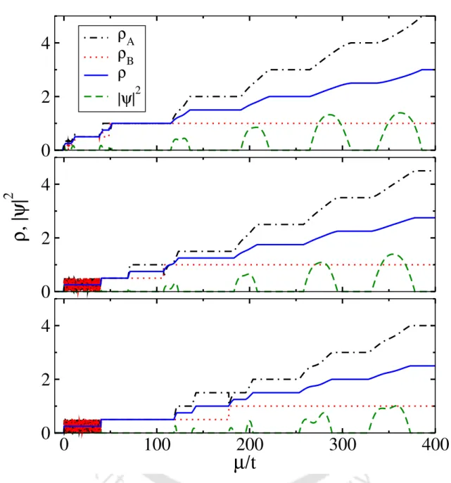
At unit filling, layer-A is in the MI phase, as the UA is sufficiently strong. We call this phase as the MIr3 phase as depicted in the phase diagram of Fig. At this stage, further increase in the value of µ will facilitate the addition of layer-B bosons, which saturate at unity filling due to the hardcore nature of the bosons.

This situation corresponds to the MI4 phases in the phase diagram where the total density of the system is ρ = 1.

Figure 3.3: Variation of ρ(solid blue curve) and |ψ| 2 (dashed green curve) with respect to µ/t for λ = 10, 70, 140 shows the gapped and gapless phases when layer-B has HCBs

Three-body constraint for bosons in layer-B

We follow the nomenclature of density distributions in Table 3.1 and discuss the phase diagram in the following text. In case (i), the particle always ends up in the deeper potential well with a smaller number of particles. Further increase of λ leads to the MIr2 phase, where the particles live in the deep locations.

Each state shows the density distribution in the supercell corresponding to a particular MI state for a given nand ρ.

Figure 3.6: CMFT phase diagram in the µ/t vs. U/t plane when bosons in layer-A are softcore and in layer-B are three-body constrained

Phase diagram in one dimension

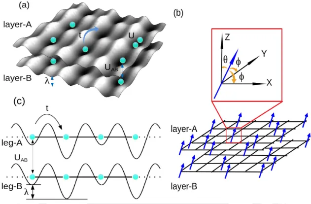
We use the DMRG method to solve the model (Eq. 3.1)) in the canonical ensemble to calculate the ground state energy and wave function. We obtain the ground state phase diagram for both the cases with bosons of leg-B separately HCBs and TBCs, while bosons in leg-A are soft-core in nature shown in Fig. When bosons are in leg-B HCBs, we take the MI point positions first increase and then decrease as in Fig.

For λ = 22, all the sites of leg-A are occupied by two particles each, while leg-B exhibits a finite density oscillation corresponding to.

Figure 3.9: Finite size scaling of chemical potentials for ρ = 1.5 for different values of λ corresponding to the phase diagram of Fig

Conclusions

In the previous chapter we studied the phase transition in a non-locally coupled lattice system. For a simple model like the BH scale, the additional coupling along the scale affects a noticeable difference in the quantum phase transitions (QPTs). It has been shown that a system of strong bosons on a two-leg ladder exhibits the ladder-insulator phase signature at half-filling due to the effect of hopping between the legs [129].

On the other hand, recent studies of three-body confined bosons on a two-leg ladder with limited inter-leg interaction have revealed the dimeric rung-insulator phase [147] .

Model and approach

By allowing attractive onsite interactions for the three-body confined bosons, we study the effect of rung-hopping on the system. It should be noted that for the HCBs in leg-b, Uα=b → ∞and due to the hardcore constraint, the terms associated with Uα=b vanish in Eq. For the exploration of quantum phases, we apply both the CMFT and DMRG methods (Chapter 2) and obtain the ground state properties of this model.

We also assume equal chemical potentials for the bosons in both legs by making µa =µb =µ for the CMFT calculations.

Results

The HCB-TBC system

• CMFT results
• DMRG results

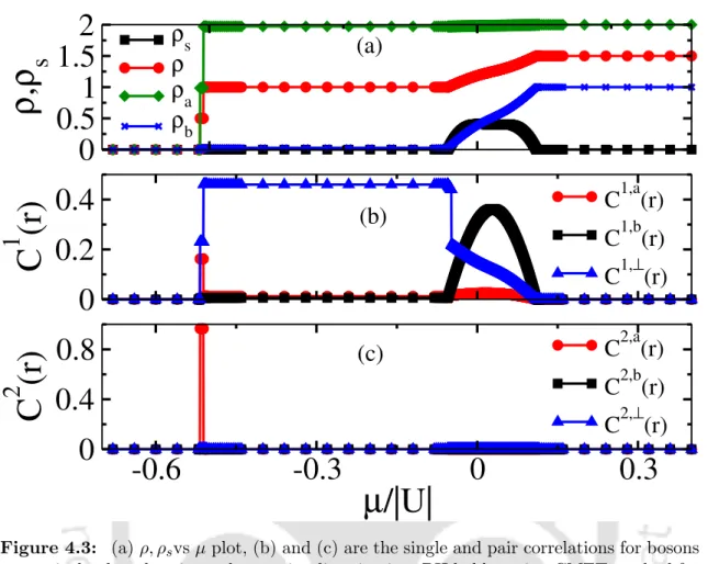
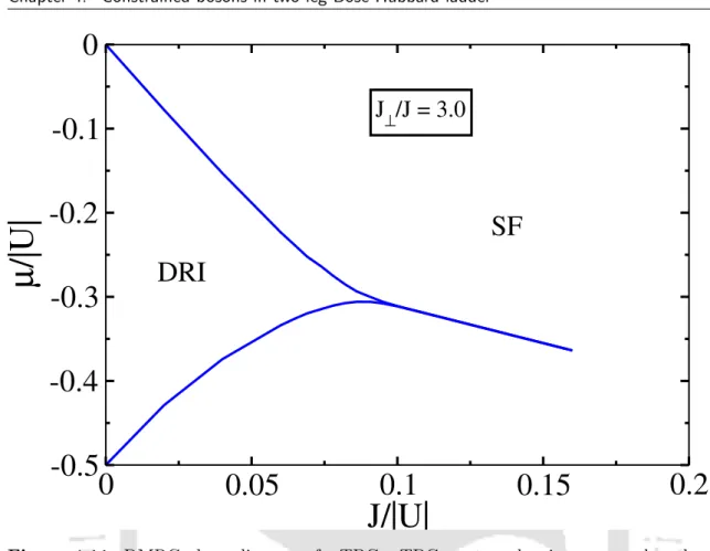
When in the SF phase, due to the TBC nature of the particles, leg-a is populated first. This is because, due to the soft-core nature of TBCs, all particles prefer to populate the a-leg in the regime of µ/|U| small. To this end, we first consider the case of J⊥/J = 3 and obtain the void phase boundaries as shown in Fig.

However, below the ρ = 1 plateau, the system density increases in two-particle steps as a function of µ/|U|, indicating a PSF phase (bottom inset of Fig. 4.8).

Figure 4.3: (a) ρ, ρ s vs µ plot, (b) and (c) are the single and pair correlations for bosons respectively along legwise and rungwise direction in a BH ladder using CMFT method for J/|U |=0.04.

The TBCs-TBCs system

Areas marked with green squares are magnified in the insets indicating the PSF phases. Note that the final values ​​of Cavg2,⊥ in the SF phase are expected due to the finite strengths of the individual particle jumps. Furthermore, in this case we find that in the regions below and above ρ = 1 the density jumps in steps of two particles as a function of µ/|U| (see insets in Figure 4.10).

This confirms the existence of the PSF phases before the system enters the full and empty states.

Conclusions

By analyzing the particle density and correlations, we validated the existence of the PSF phase using DMRG. Due to the attractive interaction between the particles, in this case we see the formation of dimers (bound bosonic pairs), which lie on the rungs of the ladder. In the many-body context, a number of such artificial atoms coupled by photons have been shown to exhibit new scenarios within the framework of the famous Jaynes-Cummings-Hubbard (JCH) model.

After this, many interesting quantum phenomena were analyzed in the framework of the JCH model [175].

Figure 4.11: DMRG phase diagram of a TBCs+TBCs system showing a gapped-gapless transition from DRI phase to SF phase

Model and method

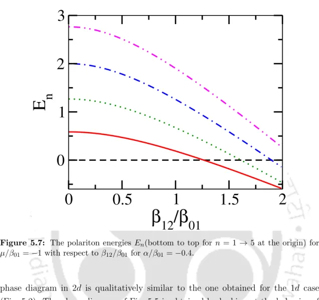
On the other hand, a recent mean-field study of a three-level equally spaced atomic system in optical cavity arrays predicts the complete suppression of the MI(1) patch after a critical β12/β01. Note that for the Λ and V systems the frequency of two transitions can be the same but require different polarizations of the photons. The removal of the higher energy levels can be implemented by using strong anharmonicity to the system [4.

To understand the effects of the strong correlations, we analyze the ground state properties of the model in Eq.

Results

Phase diagram in 1D

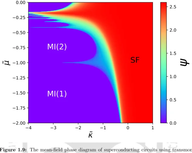
In this figure, the red solid curve delimits the boundary of the MI(2) phase, the green circles show the PSF-SF phase boundary and the black dashed curve is the vacuum state or the MI(0) phase. Moreover, in this case there is no overlap of the vacuum and the MI(2) lobe, contrary to the MFT results reported in Ref. The signature of the gapping MI(2) phase is seen as the plateaus in the ρ vs µ/β01 plot.

5.3(c) and (d) showing the signatures of the PSF and the SF phase respectively. κ/β01 plots for different system sizes of L= 20,40 and 60 to see the phase transition point.

Figure 5.2: Phase diagram of the JCH model using the DMRG method in 1d for the anharmonicity α/β 01 = −0.4

The PSF phase

This phenomenon takes place in the gapless region between the vacuum and the MI(2) phase in the regime of small κ/β01 and can therefore be called a PSF phase of polaritons. Interestingly, we also find that in the limit of two-photon propagation there exists finite correlation corresponding to the single photon and an atomic excitation which is Γatom−photon(i, j)=hσ01,i† b†iσ01,jbji. This promotes the formation of two polaritons in the transmons and indirectly the propagation of photon pair.

Therefore, the photon pair propagation and the associated polariton phase PSF in the three-level JCH model are not identical to the atomic one.

Figure 5.4: Figure shows the pair and single polariton correlation functions Γ(i, j) with distance |i − j| for ρ = 1 with (a) κ/β 01 = 0.01 and (b) κ/β 01 = 0.06

Phase diagram in 2D

The discrete jumps in the ρ−µ/β01 plot (black circles) at the two-particle steps are an indication of the PSF phase as previously discussed in Section 5.3.2 and the plateaus at ρ = 2 correspond to the MI(2) phase. This clearly shows the dominant pair correlation functions compared to the single-particle ones (see figure caption for details). Phase PSFs for both 1d and 2d systems using the DMRG and CMFT methods, respectively, as shown in Figs.

In the PSF region, discrete jumps in the density ρ correspond to a change in the polariton number of ∆n = 2, while in the SF region the polariton number changes in steps of ∆n = 1, as shown in the magnified regions shown in Figs.

Figure 5.7: The polariton energies E n (bottom to top for n = 1 → 5 at the origin) for µ/β 01 = −1 with respect to β 12 /β 01 for α/β 01 = −0.4.

Conclusions

DMRG and the CMFT approach to establish the new photon pair propagation in the system. This two-photon propagation leads to the formation of a polaritonic pair superfluid phase, which is located between the vacuum and MI(2) phases of the polaritonic phase diagram. Moving away from unit filling, we have found signatures of the superfluid phase of the pair in one leg.

The prediction of quantum phases on the two-arm Bose-Hubbard ladder model can be explored in the context of superconducting circuits.