Role of Scalar Fields in Particle Physics and Cosmology

So far, all SM predictions are in excellent agreement with experimental observations. One of the feasible solutions could be the extension of the SM of particle physics with additional fields, as they can play an important role in the universe.

Standard Model of Particle Physics

Basic set up

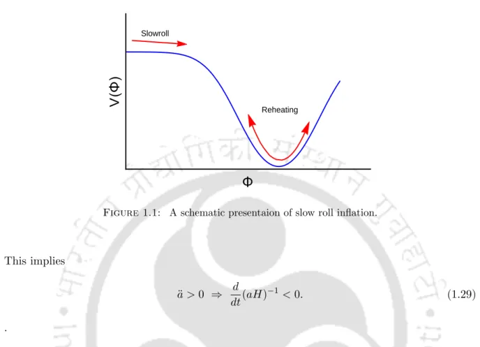
The fermion sector of the SM consists of (i) leptons (antileptons) and (ii) quarks (antiquarks). In the scalar sector of SM there is only aSU(2)Ldoublet known as Higgs (H).

Table 1.1: Field content of the SM of particle physics. The subscripts L and R represents LH and RH fields.

Success and drawbacks of the SM of particle physics

After spontaneously breaking the electroweak symmetry (SU(2)L×U(1)Y toU(1)em), the physical gauge fields can be defined as. Of these, W± and Z bosons are massive after spontaneous symmetry breaking with masses MW = gv2 and MZ = 2 cosgvθ.

Salient features of Big Bang Cosmology

Success and shortcomings of the Big Bang Cosmology

The explanation of the observed redshift or Hubble expansion, the idea of nucleosynthesis (the formation of a nucleus) and the subsequent creation of the observed abundance of light particles are among the few significant successes of big bang cosmology.

Possible resolutions of drawbacks of the Big bang cosmology and the SM of par-

Inflation

Solving the horizon and plane problems: According to equation (1.29), during inflation, the Hubble radius of motion decreases. These density perturbations are caused due to quantum fluctuations of the scalar field that drives inflation.

Dark Matter

Evidence of DM
Feasible DM candidates
Boltzman equation
Detection of DM
Real scalar singlet dark matter

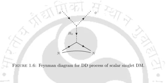
Detection of the DM is one of the greatest challenges in the modern era of particle physics and cosmological experiments. It is obvious that the probability of DM nucleon scattering increases with the size of the target and the local volume of the DM.

Figure 1.2: Galactic rotation curve for NGC 6503 shows the possible presence of the dark matter (halo) along with baryonic matter components required to match the data

Neutrino Mass

However, there are many unresolved issues, such as the nature of neutrinos (Dirac or Majorana), hierarchy of neutrino masses, and the size of CP violations in the lepton sector, etc. Note that the charged lepton mass matrix (ml) in SM is provided by Yl¯ The lLHeR term in the Yukawa Lagrangian as defined in equation (1.12).

Higgs Vacuum Stability

Higgs Vacuum Stability in Standard Model

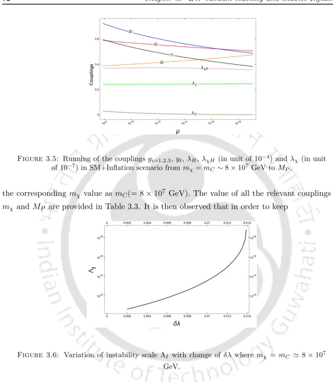
In addition, we also need to perform the renormalization group (RG) operation of the SM joins. Below we give the initial values of all SM couplings as a function of mt (top mass), mh (Higgs mass) and strong.

Figure 1.9: Running of λ h as a function of energy scale µ for [left panel:] for varying m t with fixed m H 0 = 125.18 GeV and [righ panel] for varying m H 0 with m t = 173.2 GeV

Role of scalar fields in the Universe

Outline of the thesis

A brief introduction to Supersymmetry

It is known that the quantum corrections pull the mass parameter associated with the SM Higgs field to a very high value close to the cutoff scale of the theory. This means that the supersymmetry breaking scale can be naturally generated from the strong coupling scale of the theory through small exponential suppression [260] .

Preface of the work

Then we will discuss the ISS model of dynamic supersymmetry breaking in section 2.3, followed by the role of interaction term between the two sectors in section 2.4. Modified sneutrino chaotic inflation and dynamical Supersymmetry breaking mixing coming from the current setup.

Standard sneutrino chaotic inflation in supergravity

In this work, our approach to fit chaotic inflation within the current experimental limit is to couple it to the supersymmetry breaking sector. To discuss it in detail, in the next section we present a brief overview of the ISS model of dynamical supersymmetry breaking.

SQCD sector and supersymmetry breaking in a metastable vacuum

Interaction between neutrino and SQCD sectors

Since mQ is considered smaller than Λ in the ISS setup, this situation can be achieved when the inflation field N1 satisfies N1 >[ΛMP/β]1/2. Λeff can be determined by the standard scale matching of the gauge couplings of two theories on an energy scale E = m0Q.

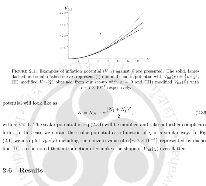
Modified chaotic potential and its implications to inflationary dynamics

In contrast, the dynamic change of the scalar potential determined by WInteff forces the ˜σ field in our case to a non-zero vacuum expectation value. To get hσi˜ in terms of ˜χ, derivative of the scalar potential with respect to ˜σ and yields. 2.35).

Results

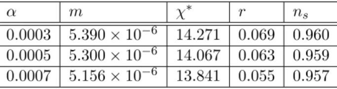
2.2, we show the corresponding points of Table 2.1 with black dots and note that those points fall within the 2σ ofns−r allowed range by PLANCK safely. The solid line for Ne= 60 shows the possible set of points (including those from Table 2.1) describing ns and r for different values of Λ.

Table 2.2: Predictions for r, n s and χ ∗ are provided for sets of values of parameters m and Λ involved in V Inf

Dynamics after inflation

This condition is easily met in our analysis of the allowed range of m, Λ, and Nc by observing that μ can be at most ∼1012 GeV for gravity-mediated supersymmetry breaking and ∼ O(1). At this stage the ISS sector stands for the breaking of supersymmetry in the metastability minimum described by equation (2.25) and hχi = 0.

It clearly shows that χ = 0 is the minimum of the potential with vacuum energy V0 = Nch2|µ|4. By introducing an additional interaction term (WInt), we can define the effective µef f in the superpotential by µ2ef f =µ2+ΛMN12.

Neutrino masses and mixing

Therefore, the light neutrino mass matrix can be obtained from the type I contribution of the saw [21] mν =mTDM1. Modified chaotic sneutrino inflation and dynamical supersymmetry breaking are the effect of renormalization group evolutions as pointed out by [294], or even other sources (e.g. type II contribution as in [295]) of the neutrino mass .

Reheating

Chapter Summary

EW vacuum stability and chaotic Higgs boson inflation mass can become large enough during inflation (meffh > HInf), the Higgs field will naturally evolve at the origin and the problem can be avoided. Below its mass scale, the inflaton can be integrated and the Higgs quartic coupling gets a shift.

Inflation Model

EW vacuum stability and chaotic inflation Similar to the original chaotic inflation model with Vφ, here too the φ field assumes a super-Planckian value during inflation. The potential is such that the χ field takes on a negative mass-squared term that depends on the field value of φ during inflation.

Inflationary Predictions

As explained below in Eq.(6), we consider αφ˜2<1.(iv) Note, however, that this term must be sufficiently large to produce significant (at least ten percent) change in r compared to the minimal chaotic inflation. Using the fact that we only keep terms of the order αφ˜2 (i.e. neglecting higher order terms), a suitable upper value of αφ˜2 can be chosen if αφ˜2 < 0.4.

Figure 3.1: Predictions for n s and r (shown in Table 3.1) as obtained from the deformed version of standard chaotic inflation are indicated by dark dots with N e = 60

Study of EW Vacuum Stability

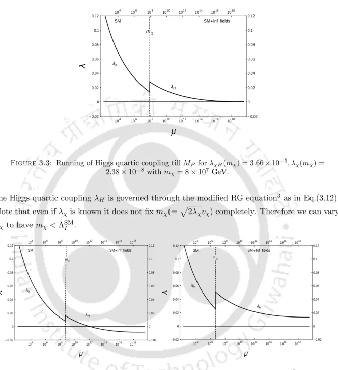
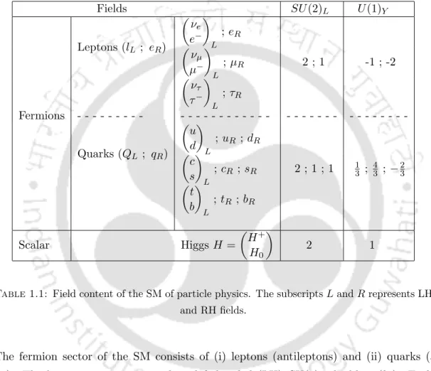
To investigate the stability of the Higgs potential after inflation, we must also take into account the λχ term from equation (3.1). With the above-mentioned scheme, we study the performance of the Higgs quaternary coupling for different mχsatisfying mχ<ΛSMI.

Table 3.2: Values of couplings in SM at m t = 173.3 GeV for m t = 173.3 GeV, m h = 125.66 GeV and α s = 0.1184.

Reheating after Inflation

Chapter Summary

The presence of the neutrino Yukawa coupling affects the operation of the Higgs-quartz coupling similar to the upper Yukawa coupling. Therefore, along with the contributions from the additional scalar fields, neutrino Yukawa coupling, Yν, is also involved in studying the operation of the Higgs quaternary coupling.

The Model

Stability of the EW vacuum in the presence of dark matter and RH neutrinos The corresponding Lagrangian part responsible for the neutrino mass is given by. Minimizing the potential V leads to the following vevs of χ and H0 (the neutral component of H), as given by.

Constraints

800 GeV, it is the NLO contribution to the W boson mass [364] that limits sinθ to a more specific range. Corrections to the electroweak precision observable via the S, T, U parameters appear to be less dominant compared to the limits obtained from W boson mass correction [364].

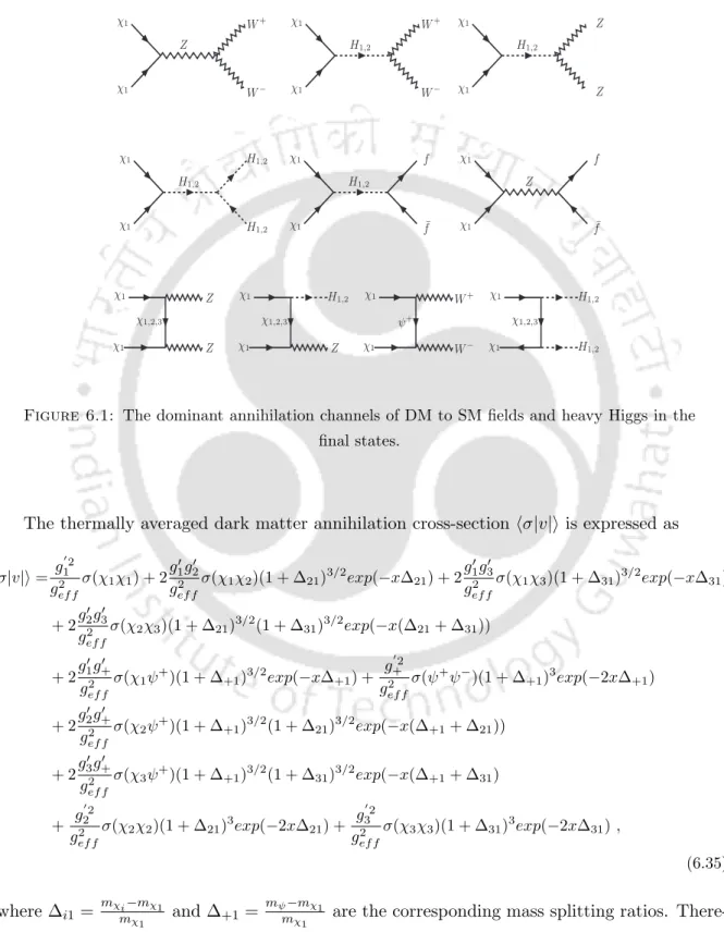
Dark matter phenomenology

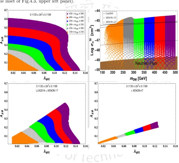
EW vacuum stability in the presence of dark matter and RH neutrinos contributing to the relic abundance satisfying the correct relic density is given at λφH−λχφ. From the top left panel of Fig.4.3, the relic density contour plot (with a particular mDM) in the λχφ-λφH plane shows that there exists a region ofλφH for which the plot is (almost) insensitive to the change in λχφ.

Figure 4.3: Top left: Allowed points on λ φH -λ χφ plane for DM having mass 150 < m DM < 500 GeV to satisfy correct order of relic density

Vacuum stability 91 provides the sinθ versus mDM plot in Fig.4.9 corresponding to residual density and LUX.

Vacuum stability

Higgs vacuum stability with right-handed neutrinos

In the presence of the RH neutrino Yukawa coupling Yν, the renormalization group (RG) equation of the SM couplings will be modified [382]. In Figure 4.11 we have shown a region plot for Tr[Yν†Yν] and mt with fixedMRat 108 GeV in terms of stability (λH remains positive until MP), metastability and instability of the EW vacuum of the SM.

Figure 4.10: RG running of λ H with energy scale µ in SM + RH neutrinos;[Left panel]:

Higgs vacuum stability from Higgs Portal DM and RH neutrinos

Finally, in Figure 4.13 we provide the region plot in Tr[Yν†Yν] -mtplane, where the stable and unstable regions are indicated by green and pink spots. This graph, compared to Figure 4.11, indicates that there is no such noticeable improvement except the mild improvement in the metastable region due to the involvement of singlet scalar (DM) with Higgs portal coupling.

EW vacuum stability in extended Higgs portal DM and RH neutrinos

Now in the combined setup of the SM, scalar DM, scalar with non-zero vev and RH neutrinos, the situation changes drastically from previous case as seen in Fig.4.16. Overall significant improvement in the stability and metstability region was observed in Tr[Yν†Yν]−mtplane compared to the earlier cases.

Figure 4.12: RG evolution of λ H with energy scale µ with SM+DM+RH Neutrinos with λ φ = 0.7, m H = 125.09 GeV and α S (m Z ) = 0.1184.: (a) [top panels]: m DM = 300 GeV, and (b) [bottom panels]: m DM = 920 GeV

Connection with other observables

Chapter Summary

On the other hand, the introduction of the RH neutrino would have a major impact on the operation of the Higgs quartic coupling due to the Yukawa neutrino interaction. Therefore we have tried here to achieve the stability of the EW vacuum in the presence of RH and DM neutrinos.

Smooth Hybrid Inflation in SQCD

Therefore, the effective mass parameter involved in equation (5.4) is determined by the relation Λ2eff = mQΛ0 and the Lagrange multiplication field is found to be proportional to the Nfth meson of the Nf = N + 1 theory. Different points on the quantum moduli space associated with this Nf =N(= 4) SQCD theory exhibit different patterns of chiral symmetry breaking.

Inflationary predictions

The search for a common origin of dark matter and inflation as a UV closed theory and also the associated scales are created dynamically. Below we briefly discuss inflationary predictions derived from this superpotential, which can limit the scales involved, Λ0,Λeff.

NGB as dark matter in SQCD

We now turn to the discussion of the interactions of these pNGBs with the SM in this structure. The interaction of pNGBs with the MSSM sector (the last term in Eq. (6.2.2)), is the Higgs-portal as:.

Relic density and direct search of pNBG DM

Negligible pNBG-LSP interaction limit

Degenerate pNBG DM
Non-degenerate pNBGs

The relic density Ω will be a function of the pNBGmG mass, coupling and α,β angles. Relic density and direct search of pNBG DM 121 The subscript n refers to the nucleon (proton or neutron).

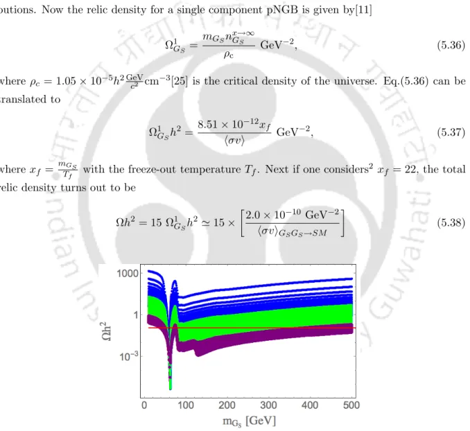
Figure 5.3: DM relic density as a function of the DM mass for the case of 15 degenerate pNBGs with tan β = 10

Non-negligible pNBG-LSP interaction limit

Relic density and direct search of pNBG DM 127, the DM relic density is still dominated by the pNBGs. The relic density for the case of 15 degenerate pNBGs as a function of pNBG DM mass is shown in Fig.

Figure 5.10: Feynman graph for Neutralino-pNBG interaction

Chapter Summary

Introduction

This is analogous to the case of supersymmetric extensions [445] where the supersymmetry breaking rate provides the dark matter mass [435]. Due to the mixing between this new scalar and the SM Higgs mat, two physical Higgs will result in this configuration.

The Model

Extended fermion sector

Therefore, including eqn (6.2) and eqn (6.3), the following mass matrix (which only includes neutral fermions) results. This can be understood later from the Lagrangian equation (6.22) which remains invariant if the dark sector fermions are odd under the remaining Z2 symmetry.

Scalar sector

However, as in our model, there exists an additional singlet scalar, φ with non-zero spin, its mixing with the SM Higgs doublet must also be included. Note that with H1 as the SM Higgs, the second term in Eq. 6.19) serves as a threshold correction for the SM Higgs quarter coupling.

Interactions in the model

Considering that all couplings involved in M are real, the elements of the diagonalization matrix V in eqn (6.5) become real[454] and thus the proportional interactions with the imaginary parts in eqn (6.22) will vanish. From equation (6.22) we note that the Largrange remains invariant if a Z2 symmetry is imposed on the fermions.

Constraints

In addition, we include the LEP bound to the charged fermions involved in the singlet-doublet model. However, in the small mixing case this turns out to be negligible [463] and can be safely ignored [432].

Dark matter phenomenology

Dark Matter relic Density

Using Eqs, the dark matter relic density χ1 can be obtained for the model parameters. The relic density of the dark matter candidate must satisfy Planck limits [39], where 1σ uncertainty is given as.

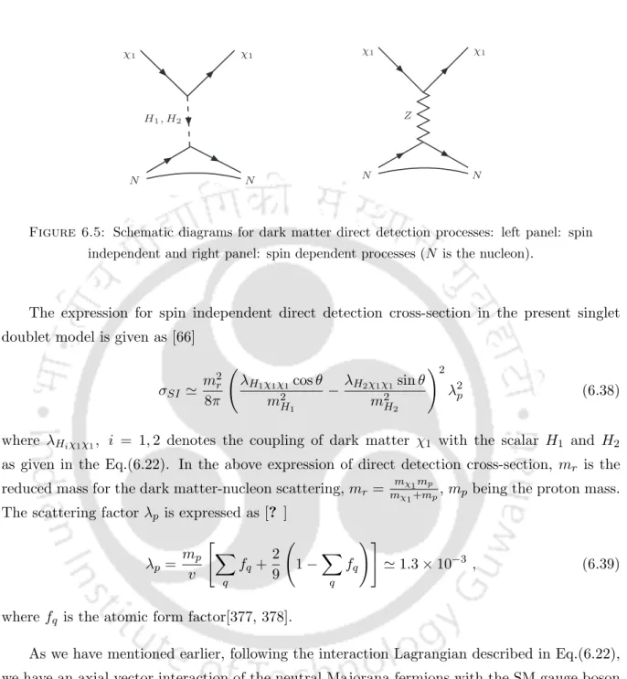
Figure 6.1: The dominant annihilation channels of DM to SM fields and heavy Higgs in the final states.

Direct searches for dark matter

In the above expression of the direct detection cross section, mr is the reduced mass for the dark matter–nucleon distribution, mr = mmχ1mp. As we mentioned earlier, after the Lagrangian interaction described in equation (6.22), we have an axial vectorial interaction of neutral Majorana fermions with the SM Z gauge boson.

Figure 6.5: Schematic diagrams for dark matter direct detection processes: left panel: spin independent and right panel: spin dependent processes (N is the nucleon).

Results

Study of importance of individual parameters
Constraining λ − sin θ from a combined scan of parameters

However, the scalar mixing has significant effect in the direct detection (DD) of dark matter. 6.8 we show the variation of the spin-independent direct dark matter detection cross section (σSI) against sinθ for the selected dark matter mass benchmark values.

Figure 6.6: DM relic density as a function of DM mass for [left panel:] m ψ = 500 GeV and [right panel:] m ψ = 1000 GeV with different choices of λ = 0.01 (blue), 0.1 (red), 0.25 (brown) and 0.4 (pink)

EW vacuum stability

On the other hand, if another deeper minimum than the EW one exists, the estimation of the tunneling probability PT from the EW vacuum to the second minimum is essential. The universe will only be in metastable state, provided the decay time is of the EW vacuum.

Phenomenological implications from DM analysis and EW vacuum stability

Therefore, all points in the green shaded region satisfy the absolute stability of the EW vacuum. The brown part of the line λ corresponds to the allowed range of the relict and DD sinθin the left (right) plane;.

Figure 6.14: Vacuum stability (green), metastable (white) and instability (pink) region in sin θ − λ plane for BP-I [left panel] and BP-II [right panel]

Chapter Summary

In Chapter 1, we provide brief introductions to the SM of particle physics and Big Bang cosmology. 171 In the 6th chapter of the thesis, we extend the minimal framework of the SDDM model with a gauge singlet scalar field.

R charges of various fields

Let ˜σ0 be the solution of this cubic part of Eq.(A.2) and its analytical form can be easily obtained (for real root). Then the scalar potential (V) in Eq. (4.1) gives rise to eleven neutral combinations of two particle states.

Table A.1: Global charges of various fields in a massless SQCD theory [259].

Numerical estimate of Boltzmann equations