We address the joint learning and scheduling problem in multihop wireless network without prior knowledge of link rates. To the best of our knowledge, it is the first distributed scheme with complexity 𝑂(1) for both learning and scheduling.
INTRODUCTION
We develop a modified version of the scheme that can be deployed in a distributed manner. In Section Ⅲ, we introduce the augmentation algorithm and incorporate it into our joint learning and planning scheme.
SYSTEM MODEL
Finally, we evaluate our schemes through simulations in Section Ⅵ and conclude our work in Section Ⅶ. In the CMAB framework, a link corresponds to an arm, a matching to superarm, and the instance link rate with the reward of the link, respectively.
ALGORITHMS
Augmentation algorithm
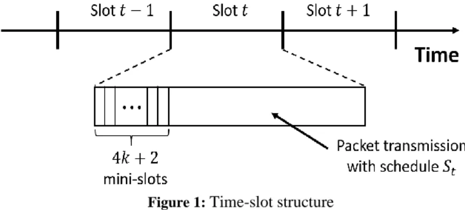
The algorithm needs two configuration parameters 𝑝 and 𝑘 and consists of the following three stages in each time slot: building extensions,. The term "active node" refers to the expansion point of an extension (there is at most one active node for each extension). Each node is selected as a seed node with probability 𝑝. a) Each seed node 𝑠 initializes its extension 𝐴𝑠. c) Each initial node 𝑠 becomes the active node 𝐴𝑠 2. a) The active node 𝑣 of each extension selects node 𝑢 in 𝑁𝐿(𝑣): 𝑢 = select_next_hop(𝑣). node 𝑣 becomes inactive and sets itself as the end station.
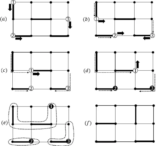
Figure 2 shows an example of the operation of the extension algorithm during a time slot 𝑡 in a 3 × 4 grid topology. The process is repeated up to a maximum of 2𝑘 + 1st mini-slot, otherwise the extension cannot be extended. the algorithm waits for 2𝑘 + 1. minislot even if not all extension can be extended before that). The node at the collision point belongs to the extension that follows the connection in 𝑆𝑡−1, as shown in Figure 2 (𝑐), where the end nodes are indicated by solid (black) number circles.
After the final operation of the 2𝑘 + 1th mini-slot, as shown in Fig.2 (𝑑), the augmentation building is completed. However, as the network scales, the probability 𝛽 of the augmentation algorithm can be very small (see Theorem 1), leading to a performance limit that is not very meaningful.
Learning through augmentation
However, this approach requires a priori knowledge of 𝜇𝑖 for each link 𝑖, which is not available in our scenarios and must be learned from 𝑋𝑖(t) that is drawn from the unknown distribution. On the other hand, the addition algorithm can serve as an approximation oracle (𝛼, 𝛽) that takes the weight 𝒘 as input, and turns out to match 𝑆 such that Pr{𝑆 ∈ 𝒮𝒘𝛼} ≥ 𝛼} =1. In this work, we develop an analysis framework that characterizes the performance of our scheme based on the augmentation algorithm and show that it can achieve the logarithmic growth of the optimal rate of 𝑘−1.
Then we denote 𝑟𝒘̅𝑡(𝑆) and 𝑟𝒘̅∗𝑡 as index sum over links in matching 𝑆 and its maximum value over all matchings, respectively. Our learning-based scheduling algorithm is shown in Algorithm 2, where for brevity we omit the subscript 𝑡 of 𝑤̂𝑖,𝑡 and 𝜏̂𝑖,𝑡. Afterwards, it calculates the index for each arm (line 7), selects matching 𝑆𝑡 with gain using the indices instead of 𝒘 (line 8), and schedules it (lines 9-10).
We develop a joint learning and scheduling scheme by plugging the augmentation algorithm into line 8 of Algorithm 2 and setting the index 𝒘̅𝑡 as the input weight. On the other hand, it no longer provides every time slot guarantee on the index sum, as the greedy algorithm does in [23].
PERFORMANCE EVALUATION
Regret performance in a single frame
Given matching 𝑆𝑡−1, 𝑤𝑒𝑖𝑔ℎ𝑡 𝒘̅𝑡, and a fixed 𝑘 > 0, the augmentation algorithm can generate a set 𝒜∗of disjoint augmentation of 𝑆𝑡−1, such that. Given any 𝑆𝑡−1, 𝑤𝑒𝑖𝑔ℎ𝑡 𝒘̅𝑡, and a fixed 𝑘 > 0, there exists 𝛿 > 0 such that the augmentation algorithm, with a probability of at least 𝛿, generates a set 𝒜∗of disjoint augmentations satisfying (𝑆 𝑡 −1 ⊕ 𝒜∗ ) ∈ 𝒮𝒘̅. The following lemma, inspired by [17], ensures that if a non-near-optimal matching in 𝒮𝒘𝛼 is played many times, its index sum is smaller than that of any near-optimal matching in 𝒮𝒘𝛼.
Δmin𝛼 ⌉ times with 𝑡-th time slot in the frame, then the probability that the total sum of UCB indices over 𝑆 at time slot 𝑡 is greater than that over any near-optimal match 𝑆′ ∈ 𝒮𝒘𝛼 bound by. The lemma shows that the augmentation algorithm can still work well even when the true weight is replaced by the UCB index. At time slot 𝑡, 𝐴𝑘-UCB randomly generates a set 𝒜𝑡 of replenishments based on the previous schedule 𝑆𝑡−1 and 𝑆𝑡−1⊕ 𝒜𝑡 is non-near-optimal.
This implies that we cannot ensure that the index sum of the chosen schedule (ie either 𝑆𝑡−1 or 𝑆𝑡−1⊕ 𝒜𝑡) is greater than 𝛼 ⋅ 𝑟𝒘̅∗𝑡 the non-comparison between the two optimal matches. We successfully solve the technical problems by considering games of non-near-optimal matches as a group.
Scheduling efficiency
DISTRIBUTED ALGORITHM
Where the equality holds due to the independence of link rates, and the last inequality holds since 𝝀 + ϵ𝟏 ∈ 𝛼Λ and therefore ∑ 𝑞𝑖(𝑡𝑛). Then, after updating the local normalizer 𝑞̃𝑣, the receiving node 𝑣 renormalizes the received reward gain as 𝐺𝑢,1′ ⋅ 𝑞̃𝑢/𝑞̃𝑣. Once the next link is determined as 𝑖 = (𝑣, 𝑛), 𝐺𝑣,1′ is calculated accordingly by adding or subtracting the average reward normalized by 𝑞̃𝑣, that is, 𝑤̂𝑖′(𝑡) =𝑞𝑖( 𝑡𝑛).
Since this repetition during the amplification phase, at the end station, we can obtain the gain from the indices normalized by 𝑞̃∗. Notes: During a frame time, the local normalization of a node is non-decreasing over time windows. In addition, two nodes in the network in the same period of time can have a different normalization value.
However, we emphasize that, given a time slot, all nodes in the same augmentation have the same value of the (local) normalizer, which is important, because the gain comparison for making a decision only takes place within an augmentation. On the other hand, as the time slot 𝑡 increases, the value of the global normalizer 𝑞∗(𝑡𝑛) is spread across the network and all local normalizers will converge to this value.
NUMERICAL RESULTS
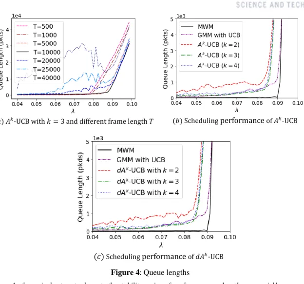
Since it is not hard to show that there exists some 𝑇′ such that all nodes 𝑣 have 𝑞̃𝑣= 𝑞∗(𝑡𝑛) with probability close to 1 for all 𝑡 > 𝑇′, we believe that 𝐐𝑴s also reach 𝐐Bs 𝑇) (even though performance and 𝑘−1. 𝑘+1Λ capacity, if the frame length 𝑇 is large enough. For comparison across frames, the regret value is set to 0 at each frame start and normalized with respect to the maximum expected reward sum 𝑟𝒘∗ within the frame. We also normalize the regret by the maximum expected reward 𝒓𝒘∗. 𝑎) 𝐴𝑘-UCB with 𝑘 = 3 and different frame length 𝑇 (𝑏) Scheduling performance of 𝐴𝑘-UCB.
This can be expected because too small a frame length leads to incomplete learning, while too large a frame length leads to a slow response to the queue dynamics. 4(𝑐) demonstrates the queue lengths of 𝐴𝑘-UCB and 𝑑𝐴𝑘-UCB, respectively, after 106 time slots, which corresponds to 200 frames. As the arrival rate gets closer to the stability region of a schedule, the queue length increases rapidly.
The service rate of each link follows a Bernoulli distribution with mean 1.2, and the packet arrival at each link is also a Bernoulli process with mean 1. Other environment settings are the same as before, except that the initial queue length is {3𝑇. The results show that while the queue lengths of 𝐴𝑘-UCB and 𝐴𝑘- UCB have stabilized, those of the index-based GMM continue to increase. Due to the high computational complexity, it is difficult to simulate MWM on larger network graphs, which is time-consuming.
CONCLUSION
In contrast, our algorithm 𝐴𝑘-UCB is analytically proven not to lead to instability for any traffic 𝝀 ∈𝑘−1. Combinatorial network optimization with unknown variables: Multi-armed bandits with linear rewards and individual observations. Distributed and provably efficient algorithms for joint channel assignment, scheduling, and routing in multichannel ad hoc wireless networks.
Stability properties of constrained queuing systems and scheduling policies for maximum throughput in multihop radio networks.
PROOF OF LEMMA 1
We also extend the definition to a set 𝒜 of disjoint gain by adding the gains, i.e. 𝐺𝑡𝒘(𝓐). The following two lemmas show that each component 𝐶 can be decomposed into small magnifications with a set of large sum links. When 𝑠𝑖𝑧𝑒(𝐶) > 𝑘, we construct a family of augmentation sets {𝒜𝑖} and show that at least one of the sets satisfies the two conditions.
After the deletions, complement 𝐶 is split into a set of disjoint complements, each of which includes at most 𝑘 links from 𝐶𝑜𝑝𝑡. Note that, in the construction procedure of {𝒜𝑖}𝑖=1𝑘+1, each link of 𝐶𝑜𝑝𝑡 is removed exactly once, and no link of 𝐶𝑡−1 is removed. Since 𝐶̂opt is obtained by removing the link of the smallest weight from 𝐶opt, it has a larger average weight than 𝐶opt, i.e. 𝑟𝒘(𝐶̂𝑜𝑝𝑡.
PROOF OF PROPOSITION 1
In general, we show that the number of explorations to a suboptimal match is bounded. For this purpose, we consider a sequence of time points where at each point a sufficiently sub-optimal match is played out. They serve as a basis for counting the total number of sub-optimal matching games.
Δmin𝛼 ⌉, and let 𝑇′ denote the first time at which all non-near-optimal matches have been sufficiently (i.e., more than 𝑙𝑇 times) explored, i.e., . Finally, the third term (19) indicates the probability of moving from a sufficiently played, non-near-optimal matching to a sufficiently played, non-near-optimal matching, and so we did just that. The total number of times non-near-optimal matchings are sufficiently played during (𝑇𝑛, 𝑇𝑛+1] is bounded by.
Taking the expectation on (15), we can obtain the expected total number of times that sub-optimal matches are selected up to time 𝑇′(≤ 𝑇). This provides a bound on the number of times non-near-optimal matches are selected up to 𝑇′.
PROOF OF LEMMA 1
PROOF OF PROPOSITION 2
Next we define 𝒮̅(𝑡) = {𝑆 ∈ 𝒮̅𝒘𝛼 | 𝜏̂𝑆, Non-near-optimal planned matches. To apply the decomposition inequality (9), we need to estimate the expected value of ∑𝑆∈𝒮̅𝒘𝛼𝜏̂𝑆,𝑇′, which can be written as. Since the future schedule 𝑆𝑡 is either 𝑆𝑡−1 and 𝑆′ according to the algorithm, we divide the event {𝑆𝑡∈ 𝒮̅𝒘𝛼} into three sub-cases based on 𝑆𝑡−' and the pro ability .
Since 𝜏̂𝑆(𝑡) ≥ 𝑙𝑇 for all 𝑆 and 𝑡 ∈ (𝑇′, 𝑇), Lemma 2 provides an upper bound 2|ℒ|𝑡−2 on each conditional probability terms in the second and third.
![Fig. 5 shows that in a certain scenario, the index-based GMM has poor performance. Motivated by [13], we consider a 6-link ring topology, where the links are numbered from 1 to 6 in a clockwise direction](https://thumb-ap.123doks.com/thumbv2/123dokinfo/10495990.0/26.892.268.639.410.686/scenario-performance-motivated-consider-topology-numbered-clockwise-direction.webp)
