Basic Research Report 18-28
Green energy research: Study of grid stability with the increasing penetration of variable renewable energy
Sangmin Cho & Ilhyun Cho
Research Staff
Head Researcher: Sangmin Cho, Research Fellow Ilhyun Cho, Associate Research Fellow Research Associates: Jaegyun Ahn, Research Fellow Outside Participants: Wooyoung Jeon, Assistant professor, Chonnam National University Sung-kwan Joo, Professor, Korea University
Juyoung Chong, Korea University
Jinyeog Lee, Korea University
Jungyoon Mo, Korea Institute for Industrial Economics & Trade
Research paper series created in collaboration with the National Research Council for Economics, Humanities and Social Sciences (NRC)
“Green energy research: Study of grid stability with the increasing penetration of variable renewable energy”
1. Collaborative research paper series
Serial no. Title of research Research institute
18-69-01
Green energy research: Study of grid stability with the increasing penetration of variable renewable energy
Korea Energy Economics Institute
2. Research participants
Research institution Head Researcher Research Associates
Hosting research institution
Korea Energy
Research Institute
Sangmin Cho, Research fellow
Ilhyun Cho, Associate research fellow
Jaegyun Ahn, Research fellow
Collaborating research institution
Chonnam National University
Wooyoung Jeon, Assistant
professor -
Korea University Sung-kwan Joo, Professor
Juyoung Chong,
Researcher
Jinyeog Lee, Researcher Korea Institute for
Industrial Economics
& Trade
Jungyoon Mo, Research
fellow -
Abstract 1. Research Necessity and Purpose
In the energy mix, the share of solar (photovoltaic) and wind energy, which are variable renewable energy (VRE)
sources, is growing at a rapid pace as these energy sources become increasingly cost-competitive around the world.
As of 2017, VRE accounted for over 20% of the energy mix in seven countries, and if the current trend continues, half of the world’s energy mix will consist of VRE by 2050.
As the demand for clean and safe energy sources increases in the Republic of Korea, the government is actively working to expand renewable energy sources to 20% of the country’s energy mix by 2030. As most of Korea’s new energy generation facilities will be solar and wind energy generation facilities, the share of VRE in Korea’s energy mix will increase rapidly to 13.5% by 2030.
Until now, the share of VRE in Korea’s energy mix has been too small to have an effect on the overall power system. However, in consideration of the rapidly increasing pace at which solar and wind energy is expanding and the Korean government’s policy direction, we must now think about the kind of impact VRE sources might have on Korea’s energy system.
This study, which was prompted by the Korean government’s Renewable Energy 3020 implementation plan, began by examining the impact that VRE sources would have on Korea’s power system in 2030. Specifically, this paper attempts to answer the question, “How much would we have to increase the energy reserve in response to the increase in VRE sources in Korea’s power system?” Additionally, this study analyzed the effects and effectiveness of energy storage systems (ESSs), which are flexible resources, as a means of offsetting the effects of VRE sources. Lastly, we also conducted model analyses and studied the literature on technologies and policies that have been considered to address the variability issue in an effort to gain an understanding of how other countries around the world are handling VRE sources.
To ensure the credibility and practicality of the results, this study created a model power system for Korea that corresponds to the implementation scenario for Korea’s 8th Basic Plan for Long-Term Electricity Supply and Demand and the Renewable Energy 2030 goal. For this research, we also used real meteorological data for Korea.
Rather than separating the effects of solar and wind energy, we integrated them to make the conditions more realistic and increased the theoretical and policy contributions of the models. All collaborating research organizations have made efforts to conduct research under the same premise and use the same data. Varying models were used for different analytical purposes, and analyses were conducted over both one-hour and 10- minute intervals. Based on these efforts, we conducted a multifaceted examination of the possible effects of VRE sources on the power system in the future and draw policy implications.
2. Summary of Contents
In response to the increase in VRE, countries are working to secure ESSs and demanding resources, which they are expanding through policy efforts.
In this study, we conducted analyses over one-hour and 10-minute periods using the Multi-Period Super Optimal Power Flow (MPSOPF) model to study the effects of the increase in VRE on Korea’s power system when solar and wind energy are supplied according to the Renewable Energy 3020 scenario. To reflect Korea’s actual situation, we used meteorological data for Korea and incorporated the Renewable Energy 3020 implementation plan and 8th Basic Plan for Long-Term Electricity Supply and Demand to simulate Korea’s power system in 2030. Unlike previous studies, this study created a model that combines solar and wind energy and conducted a more realistic analysis of the effects of increasing both solar and wind energy in Korea’s energy mix.
Before conducting a model analysis, we analyzed the solar and wind energy generation patterns using meteorological data. This analysis revealed that the solar radiation amount and onshore wind speed have a generally weak positive correlation, while the solar radiation amount and offshore wind speed have a generally weak negative correlation. This means that offshore wind energy, rather than onshore wind energy, is better able to smooth out the variations in solar energy generation, and is therefore more likely to be advantageous for the operation of the power system.
Our analysis of the energy generation profiles of representative days by season using the MPSOPF model showed that solar and wind energy had barely any effect on base load energy sources, such as nuclear power and coal, in summer and winter, having little negative effect on the operation of the power system. However, in spring and autumn, when the supply and demand of energy are low and peaks are low, a prominent duck curve emerges, showing that solar and wind energy have a considerable effect on the base-load coal energy generation.
We also estimated the required reserve energy using the MPSOPF model. In the case of representative days in summer, the supply of solar and wind energy, according to the 3020 scenario, would increase uncertainty and variability, requiring 3.9 times more reserve energy to maintain the stability of the power system compared to when there is no solar and wind energy in the energy mix. In addition, we analyzed the effect of introducing an ESS, which is a major flexible resource, as a means of addressing issues arising from the increase in VRE. We confirmed that a 5GW ESS would effectively reduce the uncertainty and variability of renewable energy, more than halving the required reserve energy. In addition, the ESS would cause a slight increase in the electricity generated from renewable energy sources, as it promotes the use of renewable energy sources that could not be used previously due to their high variability.
We also used the MPSOPF model to analyze the effect of reserve energy price changes on the amount of reserve energy and the amount of electricity generated from renewable energy sources. When the price of Korea’s reserve energy was nearly doubled to match that of the United States, the amount of reserve energy decreased dramatically (32.1%) and the amount of electricity generated from renewable energy sources in the power system decreased.
This means that an increase in the reserve energy price causes a decrease in the demand for reserve energy, thereby increasing the operational efficiency of the power system and increasing the curtailment of renewable energy.
Based on the total operational cost, ESS generated a higher cost reduction effect at a high reserve energy price than it did at a low reserve energy price.
The analysis of reserve energy over periods of 10 minutes or less was limited under the MPSOPF model. However, since analysis of variability over periods of 10 minutes or less is necessary, in consideration of the characteristics of VRE sources, we used a different methodology (variation rate analysis) to analyze reserve energy under similar conditions as the analysis of reserve energy over one-hour periods.
The amount of reserve energy required over 10-minute periods in 2030 was calculated by selecting the largest variation based on a comparison of the extent of renewable energy variation, maximum number of accidents occurring at energy generation complexes for a single renewable energy source, and number of general energy generator accidents. As a result, the required reserve energy for 10 minutes in 2030 was calculated to be 3,200MW.
In the 3020 scenario, the largest amount of the three categories was the amount of reserve energy required to prepare for rapid fluctuations in renewable energy generation. This was the amount of variation calculated in consideration of the generation of both solar and wind energy.
However, we cannot guarantee that the calculated reserve energy amount would be required in the actual operation of the power system. This study confirms that the variations in solar and wind energy did not increase proportionally to output, and the adequate reserve energy amount changed depending on solar and wind energy output and the operating conditions of the power system. We also verified the amount of reserve energy required over a 10-minute period by season depending on the operational conditions of the power system. As a result, we confirmed that the required amount of reserve energy differed by season (2,400MW in spring, 3,000MW in summer, 3,900MW in autumn, and 3,000MW in winter).
3. Conclusion and Policy Directions
Based on the results of this study, we propose the following policy directions:
First, when the supply of VRE increases in the future, it will be necessary to review the impacts of increasing the required reserve energy. The results of the analysis conducted using the MPSOPF model showed that, if the wind and solar energy supply targets are reached by 2030, the amount of required reserve energy will increase by about 3.9 times compared to when wind and solar energy are not supplied. The results of additional analysis regarding the 10-minute period reserve amount revealed that approximately 3,200MW of reserve energy is required under the current fixed reserve system in order to prepare for rapid fluctuations in solar and wind energy output over a short period of time. With the current operational reserve for 10-minute periods of 1,500MW, this is not possible.
Therefore, if Korea does reach its 2030 target for solar and wind energy, the required amount of reserve energy will exceed the current reserve amount. It will thus be necessary to consider and review increasing the reserve energy amount.
Second, it is necessary to secure flexible resources. We confirmed that the combined supply of VRE sources and flexible resources will effectively lower the required reserve energy amount and total operational expenses.
Therefore, to effectively secure flexible resources in response to increasing the supply of renewable energy, it is
necessary to make it mandatory to secure flexible resources in the short term and improve the system in the long term in order to maintain the inflow of flexible resources.
Third, it is necessary to realize compensation for flexible resources and open an ancillary service market in the long term. Through the MPSOPF model analysis, we were able to confirm that an increase in the reserve energy price causes a decrease in operational expenses. The average price of reserve energy in Korea is KRW 3,000 per MWh, which is less than half the average price in the United States. This low price, which does not meet the opportunity cost of reserve energy, tends to devalue the compensation for flexible resources, which is much less than the benefits provided by flexible resources in reducing the variability of renewable resources. Therefore, to accelerate the entry of flexible resources into the market, it is necessary to increase the price of ancillary services, such as standby reserves and amplitude modulation reserves, to reflect the opportunity cost. In the long term, the opening of a real-time electricity market and ancillary service market would induce reasonable market prices, according to the law of markets, and also provide opportunities for generating additional profits from flexible resources. In addition, this could encourage energy suppliers to invest in flexible resources and ultimately resolve problems arising from the use of renewable energy.
Fourth, it is necessary to establish a plan for variable reserve energy generation and intraday energy generation.
As mentioned earlier, variability does not increase proportionally with solar and wind energy output. Currently, reserves are operated based on fixed reserve standards every hour. However, when renewable energy sources are increased, relatively excessive amounts of reserve energy are secured during certain time periods, creating unnecessary costs. On the other hand, the amounts of reserve energy may be insufficient at other times. Therefore, it is necessary to analyze the characteristics of the power system by hour and season, including changes in the output levels of renewable energy sources, and operate variable reserves that are appropriate for the relevant time.
In addition, it is necessary to establish an intraday generation plan for the operation of variable reserves by shortening the emergency power operation periods. Currently, the power system is operated based on a one-day- ahead generation plan and real-time emergency plan. Adding one more plan alongside these two could help ensure effective responses to short-term variability in renewable resources.
Fifth, it is necessary to conduct basic research on Korea’s offshore and onshore wind power generation patterns.
Using Korea’s meteorological data, this paper examined the differences between energy generation patterns of solar and wind energy generation locations as well as the differences between the energy generation patterns of onshore and offshore wind energy. One of the noteworthy points here is that there is a difference between the energy generation patterns of onshore and offshore energy generation locations. Supplying solar energy and onshore wind energy together would intensify the solar energy duck curve, making it difficult to operate the power system. However, offshore wind energy has a smoothing effect on solar energy generation, which would reduce the burden on the power system.
As Korea plans to focus on promoting offshore wind energy in the future, it is important to increase our understanding of the effect of offshore wind energy and solar energy on Korea’s power system by conducting accurate analyses and forecasts of offshore wind energy generation patterns. Currently, however, there is a lack of basic studies relevant to Korea’s situation, making it necessary to conduct multifaceted studies on the differences between onshore and offshore wind energy generation patterns using actual observations of energy generation data. It is also important to conduct various studies on the differences between the wind and solar energy generation patterns in Korea.
Sixth, it is necessary to improve the forecasting and control system for VRE generation. The MPSOPF model establishes an optimal generation plan one day in advance. In the analysis that was conducted using this model, the capacity for reserves increases as the forecast time is expanded. Technologically, it is clear that we need a better technology for forecasting the amount of energy generated using renewable energy sources. Systematically, as in the policy proposal provided above, the introduction of variable reserves to increase the accuracy of renewable energy output forecasts would support the calculation of reserves for a real time market that takes variability into consideration and is appropriate for the level of output from renewable resources forecast for the day.
Another measure is bidding in the renewable energy market. Allowing bidding in the renewable energy market could induce improvement of the technology for forecasting energy generation amounts. This measure would also
induce renewable energy suppliers to invest in flexible resources.
In terms of controlling energy generation amounts, it is possible to install control equipment, such as pitch control gearboxes for wind energy generation and inverters for solar energy generation, to control the output. When excessive renewable energy output causes problems in the power system, the output of certain renewable resources can be controlled and appropriate compensation provided, according to regulations, in such a way that contributes to resolving the problems in the power system.
Table of Contents
Abstract... 3 Chapter 1. Introduction ... 11 Chapter 2. MPSOPF model ... 12
1. Characteristics and reserve structure of the MPSOPF model ... 12
A. Characteristics of the MPSOPF model... 12
2. Solar PV and wind power generation prediction model ... 12
A. Selection of location and analysis of correlation between weather data by location ... 13
B. Derivation of prediction profiles of solar PV and wind by location ... 17
3. 2030 Korean Power System Model Building ... 22
A. Power system model and energy mix ... 22
B. Power demand pattern ... 24
C. Pattern of integrated solar PV and wind power generation ... 25
4. Setting scenarios for reserve analysis ... 27
Chapter 3. Analysis of reserve by hour ... 29
1. Power generation mix, generation, and reserve ... 29
2. Analysis of reserve pattern by time ... 33
4. Annual cost of power system operation ... 39
Chapter 4. Analysis of reserve in 10-minute increments ... 40
1. 10-minute renewable energy variability analysis ... 40
A. Definition of output variation rate ... 40
B. Estimation of the output variation rate of renewable energy using weather data ... 42
2. Estimation of 10-minute reserve ... 44
A. 10-minute reserve reflecting renewable energy variability ... 44
B. Dynamic analysis of reserve considering the variability of renewable energy... 47
Chapter 5. Summary and Policy Direction ... 49
1. Major findings of research ... 49
2. Policy Proposal ... 50
A. Consideration of increase in required reserve ... 50
B. Necessity of flexibility resources ... 50
C. Compensation for flexibility resources and opening of ancillary services market ... 51
D. Introduction of variable reserve and day-of planning ... 51
E. Further research on offshore and onshore wind patterns ... 52
F. Improvement of accuracy of generation forecasting and control capability ... 53
References ... 55
List of Tables
Table 2-1. 16 solar PV sites and target capacity by 2030 (MW)... 13
Table 2-2. 16 wind power sites and 2030 target capacity (MW) ... 13
Table 2-3. Estimation results of probability model for Solar PV Location No. 1 (Seoul) ... 18
Table 2-4. Estimation result of probability model at Wind Power Location No. 1 (Goseong) ... 18
Table 2-5, Adjusted R-squared of solar PV probability model by location ... 19
Table 2-6. Adjusted R-squared of wind power probability model by location ... 19
Table 2-7. Setting scenarios for renewable energy in 2030 ... 26
Table 3-1. Daily generation and reserve by scenario on a representative day in summer ... 30
Table 3-2. Daily generation cost and reserve cost by scenario on a representative day in summer ... 31
Table 3-3. Analysis of required reserve per hour by scenario on a representative day in summer ... 32
Table 3-4. Average spinning reserve prices in 2014 by ISO in the United States ... 36
Table 3-5. Optimization results using high reserve price and current low reserve price: generation and reserve 35 Table 3-6. Annual cost of power system operation by scenario: ratio relative to cost of Case 1 ... 38
Table 4-1. Comparison of methods for estimating prediction error rate ... 4140
Table 4-2. Estimation of 10-minute variation rates for solar PV and wind generation ... 43
Table 4-3. Estimation of 10-minute rate of change of renewable energy in 2030 ... 43
Table 4-4. Estimation method of 10-minute reserve ... 43
Table 4-5. Variation without smoothing effect ... 44
Table 4-6. Variation of output due to the variability of renewable energy ... 44
Table 4-7. Variation rate and 10-minute reserve by season... 47
Table 5-1. Current operating reserve ... 49
List of Figures Figure 2-1. Locations of 16 solar PV complexes ... 13
Figure 2-2. Locations of 16 wind farms ... 14
Figure 2-3. Correlation between solar radiation, wind speed, and temperature ... 15
Figure 2-4. Correlation between solar radiation and wind speed... 16
Figure 2-5. 24-hour patterns of average onshore and offshore wind speed by season ... 16
Figure 2-6. 1,000 24-hour prediction profiles for Solar PV and Wind Power Locations No. 1 ... 20
Figure 2-7. Five representative profiles of Solar PV and Wind Power Locations No. 1 ... 20
Figure 2-8. Map of the Korean Power System (104-bus system) ... 21
Figure 2-9. Composition of generation capacity by source (2017 vs. 2030) ... 22
Figure 2-10. Daily power demand pattern by season (2017 vs. 2030) ... 23
Figure 2-11. Daily pattern of onshore and offshore wind generation and total wind generation on a representative day in summer ... 24
Figure 2-12. Wind power and solar PV generation and net load pattern on a representative day in summer ... 25
Figure 2-13. Pattern of net load of solar PV-wind combination model on a representative day by season ... 26
Figure 3-1. Generation profile by scenario on a representative day in summer (1) ... 28
Figure 3-2. Generation profile by scenario on a representative day in summer (2) ... 29
Figure 3-3. 24-hour generation profile by source of generation on a representative day by season: ... 31
Figure 3-4. Average contingency and load-following reserves by scenario on a representative day in summer .. 32
Figure 3-5. 24-hour required reserve profile per hour by scenario on a representative day in summer (1) ... 33
Figure 3-6. 24-hour required reserve profile per hour by scenario on a representative day in summer (2) ... 34
Figure 3-7. Low reserve price (left) and high reserve price (right): renewables generation and required reserve 36 Figure 3-8. Reserve profile by time under low reserve price and high reserve price: Case 2_Wind and Solar .... 36
Figure 3-9. Low reserve price (left) vs. high reserve price (right): cost-saving effect of ESS ... 37
Figure 3-10. Example of estimation of annual demand pattern using the PCHIP method... 38
Figure 4-1. Definition of output variation rate... 39
Figure 4-2. Method of estimating the variation rate of renewable energy ... 41
Figure 4-3. Example of probability distribution under different confidence intervals ... 42
Figure 4-4. Example of estimation of 10-minute reserve for 2030 ... 45
Figure 4-5. Variation by level of output of renewable energy (one year) ... 46
Figure 4-6. Standard deviation of variation by level of output of renewable energy ... 46
Figure 4-7. Standard variation by level of output of renewable energy ... 46
Figure 5-1. Variable reserve responses to changes in status of power system ... 50
Figure 5-2. Generation and dispatch planning procedures for a shorter dispatch cycle (CAISO) ... 51
Figure 5-3. Limitation of renewable energy output ... 53
Chapter 1. Introduction
In its Renewable Energy 3020 Implementation Plan1 of 2017, the Korean government presented the goal of expanding the share of renewable energy, such as solar and wind power, to 20% by 2030. The expansion of renewable energy deployment is a global trend, with nations worldwide striving to expand their supplies of renewable energy. Korea plans to expand its renewable energy deployment with a focus on solar PV and wind. According to the plan, the government will supply 97% of new renewables capacity using solar PV and wind by 2030, by which time the share of variable renewable energy (VRE) of total electricity generation is projected to reach 13.5%.2
Korea’s expansion of renewable energy is quite a departure from its existing energy policy, indicating that the country’s energy policy has entered an important phase of transformation. With this change, various issues have emerged in relation to potential, the unit cost of power generation, and grid stability. As the country expands its renewable energy supply, these issues will be continually raised as important policy tasks that need to be addressed on a consistent basis.
This research aims to examine issues related to the massive introduction of variable renewable energy (VRE) into the power system and devise measures for coping with them. In terms of power grid operation, both cost efficiency and supply stability must be considered. As the growing share of VRE is expected to undermine the stability of the power supply, because of its high volatility3 and uncertainty,4 advance preparations must be made.
In the Renewable Energy 3020 Implementation Plan, the government recognized the necessity of such preemptive measures and introduced measures such as the installation of grid-connected ESSs (energy storage systems) and implementation of power-to-gas technology. In addition, the establishment of an integrated control system and improvement of the electricity market system to cope with the expansion of flexibility resources are currently being discussed.5 However, the status and issues of Korea’s power system at the time when the renewable energy (solar and wind power) deployment target is attained in 2030, especially the power grid
1 Ministry of Industry, Trade and Energy, 2017, Renewable Energy 3020 Implementation Plan
2 Ministry of Industry, Trade and Energy, 2017, Renewable Energy 3020 Implementation Plan. The share of VRE is an estimate based on the targets of the plan.
2 The quantity of electricity generation fluctuates by hour, and it is difficult to control such variation.
4 It is difficult to predict the quantity of electricity generation.
5 Ministry of Industry, Trade and Energy, 2017, Renewable Energy 3020 Implementation Plan.
operation issues associated with the expansion of VRE, need to be thoroughly considered.
To address these issues, this study aims to analyze the impact of VRE deployment on the power grid in terms of reserve and devise technological and policy instruments. To achieve these goals, this paper provides the following content. Chapter 2 reviews the domestic and overseas technological and policy options being discussed and implemented to cope with the increased VRE deployment. Chapter 3 explains the MPSOPF model used to analyze reserve by hour and discusses major preconditions, while Chapter 4 uses the MPSOPF model built in Chapter 3 to conduct a simulation of Korea’s power grid status at the time when the country achieves its 2030 target for solar and wind power deployment and derives reserve by hour. Next, Chapter 5 provides an analysis of reserve per 10 minutes, which could not be obtained using the MPSOPF model, and derives additional implications.
Lastly, Chapter 6 provides a summary of the research findings and presents policy suggestions.
This study is unique in that it provides a simulation of Korea’s power grid system at the time when the country reaches its renewable energy deployment target in 2030 and estimates the reserve in consideration of both solar and wind power. Furthermore, it uses two different models to analyze reserve by hour and derives implications for model complementarity and completion. It is hoped that this research will be utilized as a basic resource for the establishment of a power grid system capable of coping with VRE deployment, thereby contributing to the achievement of the 3020 renewable energy deployment target.
Chapter 2. MPSOPF model
This chapter discusses the structure and major premises of Multi-Period Super Optimal Power Flow (MPSOPF) as the core model for analyzing “grid stability in terms of reserves,” which this study aims to explore. The MPSOPF model is used to analyze reserves by hour, and the variability analysis model used to analyze reserves by 10-minute increment as a supplement to the MPSOPF model will be explained in greater detail in Chapter 5. Although these two models have different objects of analysis and analytic processes, this study set out to reconcile the major premises and inputs of the models in order to ensure the consistency and reliability of the research. These major premises and inputs are discussed in this chapter.
1. Characteristics and reserve structure of the MPSOPF model A. Characteristics of the MPSOPF model
The objective function of the MPSOPF is to derive a power generation plan by generator that minimizes the expected costs (sum of power generation costs and reserve costs) of operating the power system while reflecting supply and demand uncertainty. To derive an optimum electricity generation plan, a set of various constraints, including demand pattern, generators, grid stability, networks, contingency, and renewable energy variability, is used.
The MPSOPF is different from the existing SCOPF is three ways. First, while the SCOPF derives an optimum generation plan for a specific time, the MPSOPF is capable of conducting 24-hour, continuous, multi-period analysis to produce simulations of a production plan from the perspective of day-ahead scheduling. Second, as the MPSOPF can process both stochastic information and deterministic information, it enables the systematic analysis of stochastic inputs6 with uncertainty. Third, the MPSOPF model estimates the quantities of two kinds of optimal reserves—load-following reserve and contingency reserve—that are necessary to maintain power system security in uncertain situations.7
These differentiated characteristics of the MPSOPF enables analysis of the effects of cost saving generated by reduced reserve attributable to the use of flexibility resources when VRE deployment reaches a significant level. Meanwhile, this study adopted the ESS as a flexibility resource. Based on a 24-hour continuous production plan that meets the ESS charging and discharging constraints, this study analyzed the effect of energy cost reduction due to peak-load shifting as well as the effect of cost saving due to the reduction of reserve through the reduced variability of renewable energy.
2. Solar PV and wind power generation prediction model
Before building the MPSOPF model, a model for predicting the pattern of solar PV and wind power generation, which is the most important parameter, needs to be developed. Solar PV and wind power generation prediction values can be estimated using a metric
6 Such as production of variable renewable energy, demand for electricity, etc.
7 A list of constraints related to the objective function of MPSOPF is provided in Jiwoon Ahn (2016). For convenience, excerpts from Jiwoon Ahn (2016) are provided in the Appendix of this paper.
model if there is actual data on solar PV and wind power generation in Korea over time. However, as it is difficult to acquire data on actual solar and wind power generation by location, we collected past weather data, including solar radiation and wind speed, for each solar PV and wind power generation site, and used it to estimate a metric model. By applying conversion parameters, we converted the solar radiation and wind power values into solar PV and wind power generation values. The solar PV and wind power generation prediction methodology is explained in detail below.
A. Selection of location and analysis of correlation between weather data by location
To build a solar PV and wind power generation prediction model, weather data from the Weather Data Portal of the Korea Meteorological Administration8 was collected. Spanning three years (2015 to 2017), the collected data includes solar radiation (MJ/m2) and temperature by time for 16 solar PV locations and wind speed (m/s) and temperature by time for 16 wind power locations (11 onshore and five offshore).
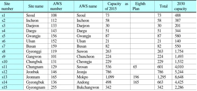
Although solar PV is currently being actively deployed largely in Jeollanam-do,9 it has been deployed relatively evenly nationwide in the form of small-scale distributed power generation facilities. Given this characteristic, this study, instead of selecting solar PV plants in specific locations, divided the entire country into 16 cities and provinces, selected a representative location10 for each city and province, and collected and analyzed weather data for each city and province. To establish a target capacity for each location for 2030, based on the deployed capacity as of 2015 and permitted capacity under the Eighth Power Supply Basic Plan,11 the installed capacity as of 2018 was estimated, and the capacities of the locations were assumed to increase in proportion to their capacities in 2018 until 2030. Table 3-2 and Figure 3-5 provide information on and the locations of the 16 solar PV sites.
Wind power, unlike solar PV, has high variation, depending on the wind in each region, which is why large wind farms are often deployed in regions with favorable wind conditions. Given this characteristic, 16 locations where large wind farms were built as of 2018 were selected as representative locations. To estimate target capacity by location by 2030, based on deployed capacity until 2015 and permitted capacity under the Eighth Power Supply Basic Plan,12 installed capacity as of 2018 was derived. The total wind power target capacity for 2030 (17,674 MW) was divided into onshore wind power (12,000 MW) and offshore wind power (5,674 MW).13 Offshore wind power was increased in proportion to the capacity of each location in 2018, and onshore wind power was evenly allocated across five locations, as there were nearly no data on capacity for the locations where wind farms have already been established. Table 3-3 and Figure 3-6 provide information on and the locations of the 16 wind farm sites.
Table 2-1. 16 solar PV sites and target capacity by 2030 (MW) Site
number Site name AWS
number AWS name Capacity as
of 2015
Eighth
Plan Total 2030
capacity
s1 Seoul 108 Seoul 73 73 488
s2 Incheon 112 Incheon 58 58 387
s3 Daejeon 133 Daejeon 30 30 201
s4 Daegu 143 Daegu 51 51 344
s5 Gwangju 156 Gwangju 87 87 580
s6 Ulsan 152 Ulsan 21 21 140
s7 Busan 159 Busan 82 82 550
s8 Gyeonggi 119 Suwon 263 263 1,754
s9 Gangwon 101 Chuncheon 224 224 1,493
s10 Chungbuk 131 Cheongju 229 229 1,532
s11 Chungnam 129 Seosan 536 65 601 4,010
s12 Jeonbuk 146 Jeonju 786 786 5,244
s13 Jeonnam 165 Mokpo 1,099 196 1,295 8,648
s14 Gyeongbuk 136 Andong 498 165 663 4,425
s15 Gyeongnam 255 Bukchangwon 342 342 2,286
8 https://data.kma.go.kr, accessed on Oct 24, 2018
9 Jeollanam-do: 24.4%, Jeollabuk-do: 17.5%. Source: Korea Energy Agency, 2017, 2016 New and Renewable Energy Deployment Statistics.
10 Seats of provincial governments and city halls
11 Ministry of Industry, Trade and Energy, 2017, Eighth Power Supply Basic Plan.
12 Indicated as “Eighth Plan” in Tables 3-2 and 3-3.
13 Ministry of Industry, Trade and Energy, 2017, Renewable Energy 3020 Implementation Plan, internal data.
s16 Jeju 184 Jeju 122 95 217 1,447 Source: author
Figure 2-1. Locations of 16 solar PV complexes
Source: author
Table 2-2. 16 wind power sites and 2030 target capacity (MW) Site
number Site name AWS
number AWS name Capacity
as of 2015
Eighth
Plan Total 2030
capacity
w1 Goseong 517 Ganseong - 583 583 801
w2 Taegisan 525 Bongpyeong 40 300 340 467
w3 Pyeongchang 526 Pyeongchang 98 476 574 788
w4 Samcheok 876 Samcheok 27 990 1,017 1,397
w5 Yeongyang 801 Yeongyang 62 301 363 499
w6 Gyeongju 859 Tohamsan 17 490 507 696
w7 Yeonggwang 769 Yeomsan 20 251 271 372
w8 Yeongheung 664 Yeongheungdo 46 - 46 63
w9 Haengwon 781 Gujwa 98 21 119 163
w10 Seongsan 792 Pyoseonmyeon 34 60 94 129
w11 Hanrim 779 Hanrim 25 192 217 298
w12 Saemangeum 700 Eocheongdo - 159 159 2,400
w13 Sinan 799 Nakwoldo 40 438 478 2,400
w14 Yeosu 931 Yokjido - - - 2,400
w15 Yeongdeok 22,106 Pohang (onshore) 40 299 339 2,400
w16 Moseulpo 855 Gapado 0 168 168 2,400
Source: author
Figure 2-2. Locations of 16 wind farms
Source: author
One of the major contributions of this study is its consideration of the integration of solar PV and wind power and examination of its impact on the power system. Previous studies analyzed either solar PV or wind power as variable renewable energy resources,14 but none analyzed both of these VRE resources at the same time. One of the purposes of this research was to look at what kind of synergy or additional issues could arise when these two energy resources are deployed together. Before such analysis, however, we will briefly introduce a correlation between solar radiation, wind power, and temperature.
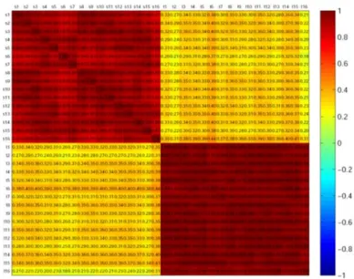
Figure 3-7 (a) is the result of an analysis of the correlation between solar radiation and temperature at 16 solar PV locations, while Figure 3-7 (b) shows the correlation between wind speed and temperature at 16 wind power locations. In these figures, a spectrum of color from red to blue indicates a correlation of 1 to -1, respectively, with green representing no correlation. They show that there is a very high correlation between solar radiation and temperature. On the other hand, the correlation between wind power and temperature is low.
In addition, as solar PV generation is concentrated in a specific period of time, because of the strong correlation of solar radiation between locations (s1 to s16), it creates a duck curve, causing problems with grid operation. The correlation of wind speed between locations (w1 to w16) is weak, and thus, nationwide, the net effect is to mitigate the variability of wind power generation (a smoothing effect).
Figure 2-3. Correlation between solar radiation, wind speed, and temperature
14 1.Jiwoon Ahn, 2016, Study on optimal generation mix of renewable energy grid integration, Korea Energy Economics Institute, basic research report, no. 16-22.
2. Wooyeong Chun, 2015, Study on building a stochastic power grid optimization model, Korea Energy Economics Institute, basic research report, no. 15-15.
(a) Correlation between solar radiation and temperature
(b) Correlation between wind speed and temperature Source: author
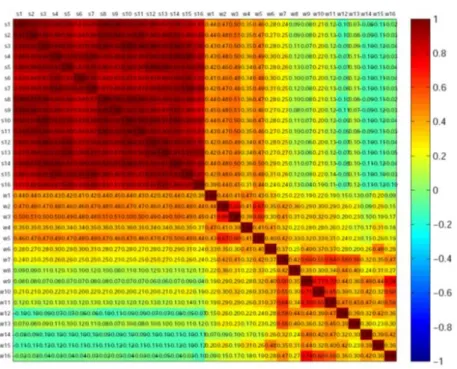
Lastly, Figure 3-8 shows the correlation between the solar radiation of the 16 solar PV locations (s1 to s16) and the wind speed of the 16 wind power locations (w1 to w16). Notably, solar radiation and onshore wind speed (w1 to w11) have an overall weak positive correlation, whereas solar radiation and offshore wind speed (w12 to w16) have a weak negative correlation. This indicates that onshore and offshore wind speed have different patterns, onshore wind speed and solar radiation have similar patterns, and offshore wind speed and solar radiation move in opposite directions. Based on these observations, the simultaneous deployment of solar PV and onshore wind power would intensify the duck curve phenomenon of the net load of solar PV, making grid operation more difficult, while the deployment of solar PV and offshore wind power together is likely to alleviate the duck curve, alleviating the problems of grid operation.
Figure 3-9 shows the 24-hour pattern of average onshore and offshore wind speed by season. Overall, wind speed in Korea is low in summer, medium in spring and autumn, and the highest during winter. Over a 24-hour period, onshore wind speed is low during the night and high in the afternoon (13 to 17). Overall, offshore wind speed remains relatively steady during the 24-hour period. In winter, when the wind speed is higher, offshore wind speed during the day is lower than that at night. This is consistent with the observation from Figure 3-8. Onshore wind speed in Korea is generally high at times of sufficient solar generation, but offshore wind speed is steady, exhibiting no correlation with solar PV. In winter, offshore wind speed moves in the opposite direction of solar
PV.
Figure 2-4. Correlation between solar radiation and wind speed
Source: author
Figure 2-5. 24-hour patterns of average onshore and offshore wind speed by season
(a) Average onshore wind speed by season (b) Average offshore wind speed by season Source: author
겨울 Winter
봄 Spring
여름 Summer
가을 Autumn
풍속 Wind speed
시간 Time
B. Derivation of prediction profiles of solar PV and wind by location
The 24-hour prediction profiles of solar PV and wind generation by location to be used as inputs for the MPSOPF model are derived using the solar radiation, wind speed, and temperature data explained earlier and by applying the method of Wooyeong Chun (2015). Wooyeong Chun (2015) presented a four-stage model for predicting solar radiation and wind power generation. This methodology is explained below.
1) Stage 1
In Stage 1, using the two-stage ARMAX model, a probability model is developed to estimate the solar radiation and wind speed for each of the 16 solar PV and 16 wind power locations.
Formula 3-1. Probability model of solar radiation and wind speed Stage 1: Deterministic Part
풍속 Wind speed
기온 Temperature
일사량 Solar radiation
Stage 2: ARMA Part
Deterministic cyclest,i: one year, half year, 24-hour cycle, 12-hour cycle, sine and cosine curves
: residual of estimation equation in Stage 1
: Stage 2 white noise residual of estimation equation
Source: author, based on Wooyeong Chun, 2015, Study on building a stochastic power grid optimization model, Korea Energy Economics Institute, Basic Research Report, no. 15-15, p.55.
Formula 3-1 shows the methodology of the probability model for estimating solar radiation and wind speed. The ARMAX model consists of two stages: Stage 1, where solar radiation and wind speed are estimated using deterministic information such as temperature and annual or daily cycle dummy variables; and Stage 2, where they are again estimated through time-series analysis based on error terms of the model from Stage 1.
Table 3-4 illustrates the results of the estimation of the probability model for solar PV locations in Seoul. The adjusted R-squared of the OLS model in Stage 1 is 76.8%, and if the ARMA model of Stage 2 is used, it rises to 95.4%.
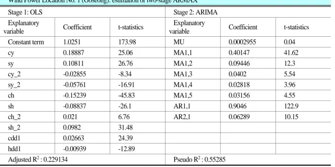
Table 3-5 shows the results of the estimation of the probability model for wind power locations in Goseong. The adjusted R- squared of the OLS model in Stage 1 is 22.9%, and when the ARMAX model of Stage 2 is used, it rises to 55.3%, which is far lower than that of the solar radiation estimation model above. Generally, the adjusted R-squared of the wind speed estimation model tends to be lower than that of the solar radiation estimation model.
Table 2-3. Estimation results of probability model for Solar PV Location No. 1 (Seoul) Solar PV Location No. 1 (Seoul): two-stage ARMAX estimation result
Stage 1: OLS Stage 2: ARIMA
Explanatory Coefficient t-statistics Explanatory Coefficient t-statistics
variable variable Constant
term 0.02834 11.09 mu 1.45E-05 0
daily cycle 0.48243 265.85 MA 1 -0.34041 -34.82
cdd 0.01423 36.29 MA 2 -0.16010 -16.21
hdd -0.00122 -6.68 MA 3 -0.06050 -7.49
AR 1 0.72454 92.46
AR 2,3 0.14544 23.77
AR 2,4 0.23966 39.9
Adjusted R2 : 0.767961 Pseudo R2: 0.954012
Source: author
Table 2-4. Estimation result of probability model at Wind Power Location No. 1 (Goseong) Wind Power Location No. 1 (Goseong): estimation of two-stage ARMAX
Stage 1: OLS Stage 2: ARIMA
Explanatory
variable Coefficient t-statistics Explanatory
variable Coefficient t-statistics
Constant term 1.0251 173.98 MU 0.0002955 0.04
cy 0.18887 25.06 MA1,1 0.40147 41.62
sy 0.10811 26.76 MA1,2 0.09446 12.3
cy_2 -0.02855 -8.34 MA1,3 0.0402 5.54
sy_2 -0.05761 -16.91 MA1,4 0.02818 3.96
ch -0.15239 -45.83 MA1,5 0.03156 4.55
sh -0.08837 -26.1 AR1,1 0.9046 122.9
ch_2 0.021 6.76 AR2,1 0.06289 10.15
sh_2 0.0982 31.48
cdd1 0.02663 24.39
hdd1 -0.00939 -12.89
Adjusted R2 : 0.229134 Pseudo R2 : 0.55285
Source: author
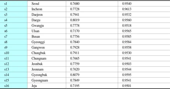
Tables 3-6 and 3-7 show the adjusted R-squared values of Stage 1 and Stage 2 in each probability model for the 16 solar PV and 16 wind power locations. On average, the adjusted R-squared of the solar radiation estimation model is 95%, but that of the wind speed estimation model is about 60% to 70%.
In summary, the analysis indicates that the adjusted R-squared of solar PV is higher than that of wind power, and the adjusted R- squared of offshore wind power is higher than that of onshore wind power. This suggests the importance of creating a wind power prediction system. In addition, the results show that offshore wind power is more predictable (lower uncertainty) than onshore wind power, giving it the advantage of promoting power grid stability. However, as the difference of R-squared was not statistically verified, interpretation of the analysis result needs to be approached with caution.
Table 2-5, Adjusted R-squared of solar PV probability model by location Location
number Location Adjusted R-squared (Stage 1) Pseudo R-squared (Stage 2)
s1 Seoul 0.7680 0.9540
s2 Incheon 0.7728 0.9613
s3 Daejeon 0.7941 0.9532
s4 Daegu 0.8019 0.9560
s5 Gwangju 0.7778 0.9518
s6 Ulsan 0.7170 0.9565
s7 Busan 0.7756 0.9585
s8 Gyeonggi 0.7840 0.9584
s9 Gangwon 0.7928 0.9558
s10 Chungbuk 0.7911 0.9530
s11 Chungnam 0.7665 0.9541
s12 Jeonbuk 0.7759 0.9503
s13 Jeonnam 0.7620 0.9544
s14 Gyeongbuk 0.8079 0.9595
s15 Gyeongnam 0.7849 0.9541
s16 Jeju 0.7195 0.9501
Source: author.
Table 2-6. Adjusted R-squared of wind power probability model by location Location
number Location Adjusted R-squared (Stage 1) Pseudo R-squared (Stage 2)
w1 Goseong 0.2291 0.5529
w2 Taegisan 0.3672 0.7599
w3 Pyeongchang 0.3798 0.6449
w4 Samcheok 0.2015 0.5467
w5 Yeongyang 0.2892 0.6150
w6 Gyeongju 0.1991 0.5839
w7 Yeonggwang 0.2046 0.7493
w8 Yeongheung 0.0790 0.7348
w9 Haengwon 0.1752 0.7887
w10 Seongsan 0.1836 0.7192
w11 Hanrim 0.1804 0.7791
w12 Saemangeum 0.1431 0.7831
w13 Sinan 0.0323 0.6588
w14 Yeosu 0.1091 0.6485
w15 Yeongdeok 0.1561 0.7844
w16 Moseulpo 0.2276 0.7952
Source: author.
2) Stage 2
In Stage 2, based on the probability model by location derived in Stage 1, we derived 1,000 prediction profiles for predicting solar radiation and wind speed using the Monte Carlo method, which involved randomly creating white noise residuals, which are error terms for each probability model in Stage 2, under the assumption of normal distribution. Correlation between locations and
correlation between solar radiation and wind speed are reflected in the creation of white noise residuals by location from the covariance-variance matrix of white noise residuals at 32 locations. As such, the derived prediction profiles by location reflect the correlation between locations. This enables an integrated analysis of two renewable energy resources (solar PV and wind) that reflects the correlation between solar PV and wind power by location.
3) Stage 3
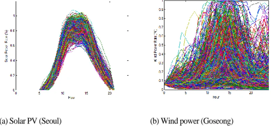
In Stage 3, the prediction profiles of estimated solar radiation and wind speed are converted into solar PV and wind power generation profiles. As for solar PV, solar radiation is converted into solar PV generation by considering the installed capacity by unit area, solar radiation-generation conversion, solar PV panel efficiency, and total capacity factor. Wind speed is converted into wind power generation by applying the IEC-315 conversion curve. Figure 3-10 shows 1,000 prediction profiles for solar PV and wind power generation at Solar PV Location No. 1 and Wind Power Location No. 1, respectively.
4) Stage 4
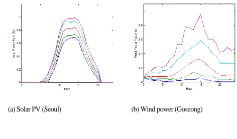
In Stage 4, five profiles were selected to represent these 1,000 solar PV and wind power generation profiles. The median of the five profiles, median ± 1 sigma, and median ± 2 sigma (the lowest and highest levels) were set. Figure 3-11 shows the five representative profiles.
Figure 2-6. 1,000 24-hour prediction profiles for Solar PV and Wind Power Locations No. 1
(a) Solar PV (Seoul) (b) Wind power (Goseong)
Source: author
Figure 2-7. Five representative profiles of Solar PV and Wind Power Locations No. 1
(a) Solar PV (Seoul) (b) Wind power (Goseong)
15 Wind power electricity generation by type of wind turbine as per the standards of the International Electrotechnical Commission (IEC).
Source: author
3. 2030 Korean Power System Model Building A. Power system model and energy mix
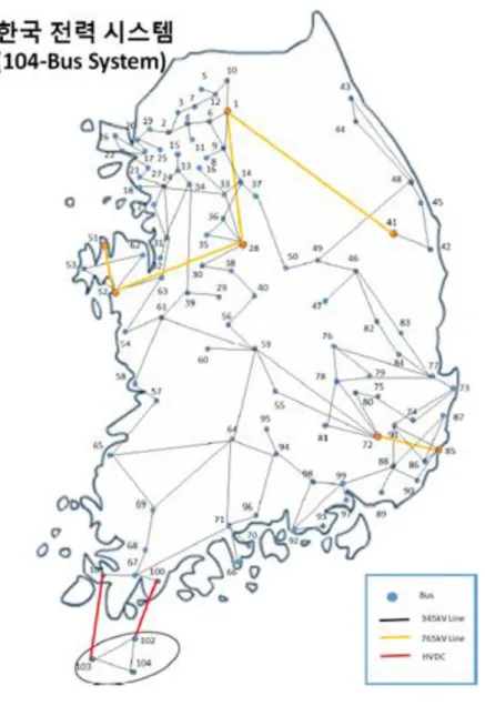
As for the framework and inputs of the Korea Power System model used in this study, the model of Jiwoon Ahn (2016) was referred to. Figure 3-12 is the map of the Korean Power System (104-bus system) created by Jiwoon Ahn (2016). The model is a 104-bus system based on transmission grids (765kV to 345kV), physical constraints of local generators, and cost function data.
Figure 3-13 compares the composition of generation capacity by source in 2017 and 2030. According to the Eighth Power Supply Basic Plan, 82% (45GW) of the capacity increase (54.6GW) from 2017 to 2030 is attributable to renewables, mostly solar PV and wind power, while the increase in capacity of conventional sources such as nuclear energy or coal is rather limited.
This study assumed that, for conventional sources such as nuclear energy, coal, LNG, and petroleum, the capacity of existing generators increases by 2030. As for solar PV and wind power generation, it is assumed that the capacities estimated for the 16 locations above are achieved by 2030. Due to the expected increase in electricity demand and expansion of renewable energy generation facilities by 2030, optimization cannot be achieved with the current power grid. Hence, this study conducts an optimization analysis without considering the power grid constraint.
Figure 2-8. Map of the Korean Power System (104-bus system)
Source: Jiwoon Ahn, 2016, Study on optimal generation mix for renewable energy grid connection, Korea Energy Economics Institute, Basic Research Report, no. 16-22, p.32.
Figure 2-9. Composition of generation capacity by source (2017 vs. 2030)
Source: author
발전용량 Generation capacity
원자력 Nuclear energy
석탄 Coal
신재생 Renewables
석유 Petroleum
양수 Pumped-storage hydroelectricity
B. Power demand pattern
Figure 3-14 shows the pattern of daily electric power demand by season in 2017 and 2030. The power demand pattern of representative days by season in 2030 is estimated under the assumption that the demand pattern of 2017 increases in proportion to summer peak load of 2030 (97.5GW) and winter peak load (100.5GW), based on the target demand of the Eighth Power Supply Basic Plan.
Figure 2-10. Daily power demand pattern by season (2017 vs. 2030)
(a) Power demand in 2017 (b) Power demand in 2030 Source: author
C. Pattern of integrated solar PV and wind power generation
Figure 3-15 shows the generation levels for 11 onshore wind power installations and five offshore wind power installations, using the same wind power installations and capacity estimated earlier, as well as the daily pattern of total wind power generation (onshore + offshore) on representative summer days.
As found earlier when examining the correlation between solar radiation and wind speed and the patterns of onshore and offshore wind speed, onshore wind speed in Korea, contrary to common sense, is lower at night and much higher during the day. This suggests that when only onshore wind power is introduced, it aids grid operation by generating more power during the day, when power demand is high, but intensifies the duck curve caused by solar PV, thus making grid operation more difficult, under the scenario of the Renewable Energy 3020 Implementation Plan that proposes the deployment of both wind and solar PV. On the other hand, offshore wind power generates a little more power at dawn than during the day.
The patterns of onshore and offshore wind power generation suggest that when wind power is deployed along with solar PV in Korea, offshore wind power has the advantage of reducing the burden of grid operation, thanks to its mitigating influence on the duck curve.
Total wind power generation, which includes both onshore and offshore wind power, shows that power generation is more influenced by offshore wind power, as this study assumed the ratio of onshore to offshore wind to be 2.1:1. Figure 3-16 illustrates the patterns of wind power generation solar PV generation, and the patterns of net load that is the difference between energy demand and electricity production from renewables. As mentioned earlier, wind power generation remains steady over time due to the large effect of offshore wind, and thus net load is not much different from the demand pattern over the entire day. On the other hand, as solar PV generation is highest during the day, the duck curve of net load becomes more pronounced. Meanwhile, although the uncertainty of solar PV is less than that of wind power, the variability of solar net load is similar to that of wind net load because the installed capacity of solar PV will be double that of wind power in 2030.
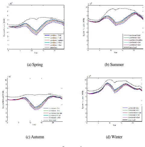
Figure 3-17 shows the seasonal net load patterns of combined solar PV and wind power generation. As peak demand is high in summer and winter, the lowest point of the duck curve is not much different from the lowest point at night. In spring and autumn, however, the lowest point of the duck curve is much lower than the lowest point at night, making it very difficult for grid operators to manage base load generation.
Figure 2-11. Daily pattern of onshore and offshore wind generation and total wind generation on a representative day in summer
(a) Onshore wind power (b) Offshore wind power
(c) Total wind power
Source: author
Figure 2-12. Wind power and solar PV generation and net load pattern on a representative day in summer
(a) Wind power generation (b) Solar PV generation
(c) Wind power net load (d) Solar PV net load Source: author
Figure 2-13. Pattern of net load of solar PV-wind combination model on a representative day by season
(a) Spring (b) Summer
(c) Autumn (d) Winter
Source: author
4. Setting scenarios for reserve analysis
Table 3-8 outlines the scenarios set up by this study to analyze the power system in 2030. This study set up seven scenarios depending on the deployment of solar PV, wind power, and ESS facilities. Among these, the core scenarios are: Case 1 (c1), Case 2_Wind and Solar (c2ws), and Case 3_Wind and Solar (c3ws). Case 1 is the base scenario, while Case 2_Wind and Solar is used to analyze the effect of solar PV and wind power on the power grid. Case 3_Wind and Solar further analyzes the effect of an ESS on the grid.
Table 2-7. Setting scenarios for renewable energy in 2030
Scenario Description of scenario Abbreviation
Case 1 Base scenario (without solar and wind) c1
Case 2_Wind Case 1 + wind (17,674MW) c2w
Case 2_Solar Case 1 + solar (33,530 MW) c2s
Case 2_Wind and Solar Case 1 + wind and solar (51,204MW) c2ws
Case 3_Wind Case 1 + wind + ESS (5GW) c3w
Case 3_Solar Case 1 + solar + ESS (5GW) c3s
Case 3_Wind and Solar Case 1 + wind and solar + ESS (5GW) c3ws Source: author
Case 1 is the standard scenario where solar PV and wind power are not introduced into the Korean power system by 2030. Case 2_Wind is a scenario where wind power is deployed until the target capacity of the Renewable Energy 3020 Implementation Plan is reached, while Case 2_Solar is a scenario where solar PV is deployed until the same target capacity is reached. In Case 2_Wind and Solar, both wind and solar PV are deployed, and in Case 3, an ESS is adopted as a flexibility resource for controlling the variability of renewable energy. Case 3_Wind is a scenario where an ESS is added to Case 2_Wind, and for Case 3_Solar, an ESS is added to Case 2_Solar. Likewise, Case 3_Wind and Solar is a scenario where an ESS is added to Case 2_Wind and Solar. Here, the ESS is assumed to be a lithium-ion battery with a capacity of 5GW (5% of peak demand) and energy volume of 15GWh that can discharge maximum power for three hours at an energy efficiency of 95%.
Besides the ESS, the flexibility resources of VRE include LNG generation, demand response, and pumped-storage hydroelectricity. This study chose the ESS as the representative flexibility resource not only because of its superior economic feasibility and technology, but also because it is currently being considered as a major flexibility resource in many countries and it makes analysis easier under the MPSOPF model.
This study aims to make the following four contributions by establishing the MPSOPF model and scenarios and analyzing the impact of VRE on the power system at the time when the renewable energy deployment target for 2030 is reached. First, this study provides information on the required reserve for day-ahead planning at the time when the renewable energy deployment target for 2030 is achieved. Second, it analyzes contingency reserve, which reflects uncertainty within time, using a multi-period optimization analysis and load-following reserve, which reflects variability between times. Third, it examines the change in the required reserve amount when the reserve price rises and analyzes the trade-off relationship between the reserve cost spent to address the variability and uncertainty of renewable energy and cost of energy lost by not using renewable energy. Based on this, the importance of setting an appropriate reserve price is reviewed. Fourth, this study analyzes the necessity and effect of flexibility resources by reviewing the effect of substituting reserve with flexibility resources (ESS) as backup facilities for renewable energy as well as the cost-saving effect of reducing reserve and energy generation.
Chapter 3. Analysis of reserve by hour 1. Power generation mix, generation, and reserve
Figures 4-1 and 4-2 show 24-hour generation profiles by source of generation on a representative day in summer based on the performance of the MPSOPF optimization of the seven scenarios established in this study. In Case 1, hydro (blue), nuclear (red), and coal (yellow) provide base-load generation, while combined-cycle power (sky blue), gas turbine (gray), and heavy oil (brown) handle peak load.16 Wind is indicated in blue, and solar PV in green.
In Case 2_Wind, wind power produces electricity steadily throughout the entire day, replacing gas turbine and heavy oil as sources of generation for handling peak load. In Case 2_Solar, solar PV in summer increases generation during peak-load hours, creating a duck curve, replacing peak-load generation, and approaching the base-load generation sources such as coal-fired generation (Figure 3-1). In Case 2_Wind and Solar, the core scenario of this study, renewable energy generation is concentrated during peak-load hours, replacing a portion of coal-fired generation (Figure 3-2).
In Case 3, where an ESS is added, variability and reserve cost are reduced through the smoothing of the net-load pattern. The ESS stores energy at a lower cost during hours of high renewable energy generation, and discharges that energy during hours when the marginal cost of electricity production is high, leading to reduced generation cost.
Figure 3-1. Generation profile by scenario on a representative day in summer (1)
Case 1
Without solar PV and wind
Case 2_Wind Wind only (17,674MW)
Case 2_Solar Solar PV only (33,530MW)
16 The sums of load-following up reserve, load-following down reserve, and contingency reserve under Case 1 and Case 2_Wind and Solar are compared.
Case 3_Wind Wind only + ESS (5GW)
Case 3_Solar Solar PV only + ESS (5GW) Source: author
Figure 3-2. Generation profile by scenario on a representative day in summer (2)
Case 2_Wind and Solar Solar PV and wind (51,204MW)
Case 3_Wind and Solar
Solar PV and Wind (51,204MW) + ESS (5GW) Source: author
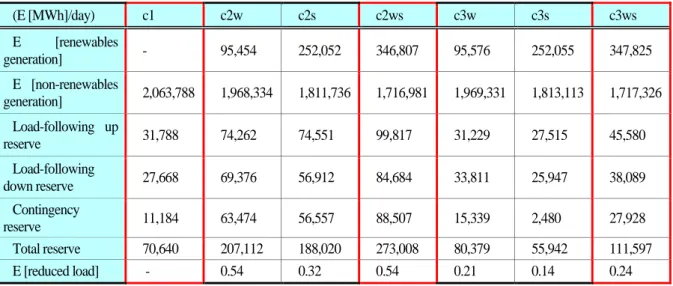
Table 3-1 shows the optimization of generation and reserve by scenario on a representative day in summer. A comparison of Case 1 and Case 2_Wind and Solar shows that the reserve increased by nearly 3.9 times. That is, the deployment of sufficient wind and solar PV generation to reach the renewable energy target for 2030 would effectively replace coal-fired generation; however, because of the high uncertainty and variability of VRE, the amount of reserve necessary to maintain the stability of the power system is almost four-times greater than in the scenario where wind and solar PV are not deployed. Hence, a sufficient amount of reserve needs to be secured in order to prepare for the increased penetration of VRE. If Case 2_Wind and Solar is compared to Case 3_Wind and Solar, the use of an ESS (5GW) as a flexibility resource is found to effectively mitigate the uncertainty and variability of VRE, reducing the required reserve by half. Furthermore, as the ESS alleviates the variability of renewable energy, renewable energy facilities that had been rejected by the power grid due to their high variability can be now integrated into the grid, leading to a moderate increase in renewable energy generation. In other words, flexibility resources not only help secure the stability of power system operation, but also contribute to the increased integration of renewable energy into the power system, boosting the profitability of renewable energy projects and encouraging investors to enter the market.
Table 3-1. Daily generation and reserve by scenario on a representative day in summer
(E [MWh]/day) c1 c2w c2s c2ws c3w c3s c3ws
E [renewables
generation] - 95,454 252,052 346,807 95,576 252,055 347,825 E [non-renewables
generation] 2,063,788 1,968,334 1,811,736 1,716,981 1,969,331 1,813,113 1,717,326 Load-following up
reserve 31,788 74,262 74,551 99,817 31,229 27,515 45,580 Load-following
down reserve 27,668 69,376 56,912 84,684 33,811 25,947 38,089 Contingency
reserve 11,184 63,474 56,557 88,507 15,339 2,480 27,928
Total reserve 70,640 207,112 188,020 273,008 80,379 55,942 111,597
E [reduced load] - 0.54 0.32 0.54 0.21 0.14 0.24
Source: author
Table 3-2 shows the cost of 24-hour generation and reserve by scenario on a representative day in summer. As with the results shown in Table 3-1, comparing Case 1 to Case 2_Wind and Solar, as renewables replace thermal power generation, the reduced use of fossil fuels leads to a significant reduction in generation costs;17 however, the high variability of wind and solar PV results in the reserve cost rising by 386%. Meanwhile, comparing Case 2_Wind and Solar to Case 3_Wind and Solar, the introduction of an ESS significantly reduces the required reserve and causes a moderate decline in the generation cost, as additional renewables are integrated into the grid. As a result, the total operation cost falls by 1.2% with the introduction of an ESS (5GW).
Table 3-2. Daily generation cost and reserve cost by scenario on a representative day in summer
(E [million KRW/day]) c1 c2w c2s c2ws c3w c3s c3ws
E [generation cost] 75,565 68,266 56,947 50,590 68,226 56,976 50,425 Load-following up reserve
cost 94 219 218 292 92 81 133
Load-following down
reserve cost 80 202 167 248 98 76 112
Contingency reserve cost 33 186 166 259 45 7 82
E [storage inefficiency cost] - - - - 13 11 30
E [total operation cost] 75,772 68,872 57,498 51,389 68,473 57,152 50,782 Source: author
Figure 3-3 illustrates the 24-hour generation profiles of Case 2_Wind and Solar on a representative day by source of generation and by season. In spring and autumn, when power demand is low and peak load is flat, solar PV generation makes the duck curve more pronounced and significantly influences coal-fired generation (base load). On the other hand, in winter, when peak demand is high and solar PV generation is relatively low, net load is larger. However, even in spring and autumn, solar PV and wind generation are not expected to affect nuclear power generation by 2030. Accordingly, stable grid operation is likely possible through the active buildup of reserve. However, as these analysis results are based on information currently available, the actual amount of required reserve in 2030 and the impact of renewables on grid operation need to be based on up-to-date information of that year.
Figure 3-3. 24-hour generation profile by source of generation on a representative day by season:
Case 2_Wind and Solar
(a) Spring (b) Summer
17 Generation cost refers to energy cost and is not the same as the unit cost of generation. Energy cost includes only variable cost. Accordingly, a decline in generation cost does not translate to a reduction in consumers’ bills.
(c) Autumn (d) Winter Source: author
2. Analysis of reserve pattern by time
Table 3-3 shows the amount of reserve per hour by scenario on a representative day in summer. In Case 1, the amount of average required reserve per hour is 3,051MWh, but in Case 2_Wind and Solar, it rises significantly to 11,765MWh. In Case 3_Wind and Solar, where an ESS (5GW) is introduced, the average required reserve per hour declines significantly to 4,850MWh.
Meanwhile, in Case 2_Wind and Solar, the maximum reserve is 20,105MWh, and the minimum reserve is 3,063MWh, revealing a significant variation in required reserve by time.18 Figure 3-4 shows the average load-following reserve and average contingency reserve by scenario, indicating that, when VRE is deployed in a large scale, the load-following reserve is larger than the contingency reserve.
Table 3-3. Analysis of required reserve per hour by scenario on a representative day in summer MWh/
hour
Load-following reserve Contingency reserve Sum of
average reserves
Average Max Min Average Max Min
c1 2,585 6,643 40 466 466 466 3,051
c2w 6,245 8,914 2,432 2,638 3,712 1,051 8,883
c2w 5,716 10,742 40 2,439 5,154 466 8,155
c2ws 8,022 13,196 2,100 3,743 6,909 963 11,765
c3w 2,828 6,835 - 641 2,414 - 3,469
c3s 2,324 5,588 - 108 1,439 - 2,432
c3ws 3,638 8,243 - 1,212 4,539 - 4,850
Source: author
Figure 3-4. Average contingency and load-following reserves by scenario on a representative day in summer
18 Sum of maximum load-following reserve and maximum contingency reserve and sum of minimum load-following reserve and minimum contingency reserve.
Source: author
Figures 4-5 and 4-6 show the 24-hour reserve profiles per hour for up and down reserves. In Case 1, where uncertainty is low overall, at times when power demand increases or decreases, only a small amount of load-following reserve is needed. Case 2_Wind and Solar is similar to Case 2_Solar and requires higher reserve per hour on the whole.
In Case 3, overall, the required reserve by time dropped remarkably and effectively. However, Case 3_Wind and Solar shows that a certain level of reserve is necessary, especially during peak demand hours, suggesting that additional ESSs are needed.
Figure 3-5. 24-hour required reserve profile per hour by scenario on a representative day in summer (1)
Case 1
Case 2_Wind Case 2_Solar
Case 3_Wind Case 3_Solar Source: author
Figure 3-6. 24-hour required reserve profile per hour by scenario on a representative day in summer (2)
Case 2_Wind and Solar
Case 3_Wind and Solar Source: author