JHEP02(2016)047
Published for SISSA by Springer
Received: November 11, 2015 Accepted: January 1, 2016 Published: February 8, 2016
Brane brick models, toric Calabi-Yau 4-folds and 2d (0,2) quivers
Sebasti´an Franco,a,b Sangmin Leec,d,e,f and Rak-Kyeong Seongg
aPhysics Department, The City College of the CUNY, 160 Convent Avenue, New York, NY 10031, U.S.A.
bThe Graduate School and University Center, The City University of New York, 365 Fifth Avenue, New York NY 10016, U.S.A.
cCenter for Theoretical Physics, Seoul National University, Seoul 08826, Korea
dDepartment of Physics and Astronomy, Seoul National University, Seoul 08826, Korea
eCollege of Liberal Studies, Seoul National University, Seoul 08826, Korea
fSchool of Natural Sciences, Institute for Advanced Study, Princeton, NJ 08540, U.S.A.
gSchool of Physics, Korea Institute for Advanced Study, Seoul 02455, Korea
E-mail: [email protected],[email protected],[email protected]
Abstract: We introduce brane brick models, a novel type of Type IIA brane configura- tions consisting of D4-branes ending on an NS5-brane. Brane brick models are T-dual to D1-branes over singular toric Calabi-Yau 4-folds. They fully encode the infinite class of 2d (generically)N = (0,2) gauge theories on the worldvolume of the D1-branes and stream- line their connection to the probed geometries. For this purpose, we also introduce new combinatorial procedures for deriving the Calabi-Yau associated to a given gauge theory and vice versa.
Keywords: Brane Dynamics in Gauge Theories, Supersymmetric gauge theory, D-branes ArXiv ePrint: 1510.01744
JHEP02(2016)047
Contents
1 Introduction 2
2 2d (0,2) theories from D1-branes over toric CY4 cones 3 2.1 Unification of quiver and toric J- and E-terms: periodic quivers 4 2.2 Earlier constructions: brane box models for orbifolds 6
3 Brane brick models 8
3.1 Brane brick models as type IIA brane configurations 8
3.2 The brane brick model — gauge theory dictionary 9
3.3 Mass terms and higgsing 12
4 Brane brick models from geometry 14
4.1 Amoebas and coamoebas 14
4.2 Periodic quivers from coamoebas 17
5 Geometry from brane brick models 21
5.1 Phase boundaries and brick matchings 22
5.2 A combinatorial definition of brick matchings 25
5.3 A correspondence between GSLM fields and brick matchings 27 5.4 The fast forward algorithm for brane brick models 28
6 Partial resolution 29
6.1 CY3 partial resolution and zig-zag paths 29
6.2 CY4 partial resolution and phase boundaries 30
7 Brane brick models for CY3 ×C theories 33
7.1 Dimensional reduction 33
7.2 Brane brick models from brane tilings 34
7.3 Examples 37
7.3.1 C ×C 37
7.3.2 SPP×C 41
8 Beyond orbifolds and dimensionally reduced theories 43
8.1 Brane brick models from global symmetries 44
8.2 Examples 45
8.2.1 D3 brane brick model 45
8.2.2 Q1,1,1 brane brick model 49
9 Conclusions 51
A The fast forward algorithm: C4/Z2×Z2×Z2 54
B Hilbert series and plethystics 58
B.1 Hilbert series for the D3 theory 60
B.2 Hilbert series for the Q1,1,1 theory 62
JHEP02(2016)047
1 Introduction
In recent years, there have been intense efforts in mapping the landscape of quantum field theories and uncovering their dynamics. As part of this enterprise, quantum field theories in various dimensions and with diverse amounts of supersymmetry have been investigated and connections between many of them have been explored.
This article is devoted to 2dN = (0,2) theories, which are particularly interesting for various reasons. Despite the reduced amount of SUSY, chirality and holomorphy provide substantial control of their dynamics. The recent discovery of a new IR equivalence between different theories known as triality [1] is an interesting example of this. In addition, these theories arise on the worldsheet of heterotic strings. Another exciting development is the geometric realization of a wide class of these theories via compactification of the 6d (2,0) theory on 4-manifolds [2].
It is extremely desirable to understand how to engineer 2d(0,2) gauge theories in terms of branes. Early steps in this direction were taken in [3–5]. This question was revived in our previous work [6], which initiated an ambitious program aimed at understanding in detail the infinite class of gauge theories arising on D1-branes probing arbitrary singular toric Calabi-Yau (CY) 4-folds and developing T-dual brane setups.1
The part of the story regarding D1-branes on toric CY4 singularities was completely developed in [6]. In particular, an algorithm for connecting gauge theories to the probed geometry, which arises as the their classical mesonic moduli space, was developed. We referred to it as the forward algorithm. In addition, a systematic procedure for obtaining the gauge theory for an arbitrary toric CY4 singularity by means of partial resolution was introduced.
In this work, we will fully develop the second part of the story: the T-dual brane setups.
These brane configurations are called brane brick models and their basic features were already anticipated in [6]. They substantially simplify the connection between geometry and gauge theory.
This article is organized as follows. Section 2 reviews general features of the gauge theories on D1-branes over toric CY4 folds, their description in terms of periodic quivers and the brane box configurations for abelian orbifolds of C4. Section 3 introduces brane brick models and presents the dictionary connecting them to gauge theories. Section 4 introduces the fast inverse algorithm, for going from the toric diagram of a CY4 to the corresponding brane brick model. Section 5 presents the fast forward algorithm, which goes in the opposite direction and determines the CY4 associated to a brane brick model.
A key ingredient of this approach is a correspondence between GLSM fields and a new class of combinatorial objects, denoted brick matchings. This combinatorial computation of the geometry represents a tremendous simplification over the standard forward algorithm of [6]. Section6discusses partial resolutions in terms of brane brick models, extending the comprehensive study presented in [6]. Section 7 is devoted to Calabi-Yau 4-folds of the form CY3×C. The corresponding 2dgauge theories have (2,2) SUSY and can be obtained from the 4d N = 1 theories associated to the CY3 by dimensional reduction. A lifting
1Other interesting approaches to the D-brane engineering of 2d(0,2) theories can be found in [7–9].
JHEP02(2016)047
algorithm for generating the brane brick model for the 2d theory from the brane tiling for the 4d one is introduced. Section 8 goes beyond orbifolds and dimensionally reduced theories and studies the brane brick models for generic toric CY4 singularities. Section 9 presents our conclusions and some directions for future research.
2 2d (0,2) theories from D1-branes over toric CY4 cones
For a thorough discussion on the structure of general 2d (0,2) theories, including their supermultiplet structure and the construction of their Lagrangians in terms of (0,2) su- perspace, we refer to [1,3,7,10]. This paper focuses on 2dtheories on the worldvolume of D1-branes probing toric Calabi-Yau (CY) 4-folds. As explained in [6], these theories have a special structure which is the reason for their beautiful connection to toric geometry and to certain combinatorial objects that are going to be introduced in this paper.
Symmetries and quivers. D1-branes probing a generic toric CY4 singularity preserve (0,2) SUSY. When the CY4 is of the form CY3×C, CY2×C2 and C4, there is a non- chiral enhancement of SUSY to (2,2), (4,4) and (8,8), respectively. Such theories can be constructed by dimensional reduction from 4dN = 1, 2 and 4. Chiral SUSY enhancement to (0,4) occurs for CY2×CY2. Finally, enhancement to (0,6) and (0,8) is possible for certain orbifolds [3].
The gauge symmetry and matter content of these theories can be encoded in terms of generalized quiver diagrams involving two types of matter fields in bifundamental or adjoint representations: chiral and Fermi multiplets. The gauge group for these theories is a product of U(Ni) factors. As usual, each of these factors is represented by a node in the quiver. The total number of gauge nodes in the quiver is given by the volume of the toric diagram normalized with respect to a minimal tetrahedron.
All matter multiplets are in adjoint or bifundamental representation of the gauge group.
Chiral multiplets are represented by oriented arrows in the quiver diagram. We typically label the chiral fields asXij withiandj gauge node indices. Fermi multiplets are labeled similarly, Λij, but they are represented by red unoriented lines in the quiver diagram. The reason for this is that 2d(0,2) theories are invariant under the exchange of any Λij with its conjugate ¯Λij, i.e. Fermi fields are intrinsically unoriented.
Anomalies. Cancellation of SU(Ni)2 gauge anomalies imposes severe constraints on 2d (0,2) theories.2 Throughout this paper we will restrict to the case of N regular D1-branes, for which all nodes are U(N). More general rank assignments are possible in the presence of fractional D1-branes. For the case when all ranks are equal, Ni = N, cancellation of SU(Ni)2 anomalies at nodeirequire
nχi −nFi = 2, (2.1)
wherenχi and nFi are the total number of chiral and Fermi fields that are attached to node i, respectively. Adjoint chiral or Fermi fields contribute 2 tonχi ornFi , respectively.
2In theories on D1-branes at singularities, abelian gauge anomalies are cancelled by a generalized Green- Schwarz mechanism through interactions with bulk RR fields [11].
JHEP02(2016)047
Toric J- and E-terms. In a general 2d(0,2) theory, every Fermi field Λij is associated with a pair of holomorphic functions of chiral fields: Eij(X) (with the same gauge quantum numbers of Λij) andJji(X) (with conjugate gauge quantum numbers) [1,3,7,10]. In the theories dual to toric Calabi-Yau 4-folds, these functions take a very special form. This restriction was called the toric condition in [6], and implies that J- and E-terms take the following general form
Jji=Jji+−Jji−, Eij =Eij+−Eij−, (2.2) whereJji± and Eij± are holomorphic monomials in chiral fields.
CY4 geometry from gauge theory. The CY4 geometry probed by the D1-branes is recovered as the classical mesonic moduli space of the gauge theory that lives on the worldvolume of the D1-branes. Given that the mesonic moduli space of the worldvolume theory of a stack ofN D1-branes is theN-th symmetric product of the worldvolume theory on a single D1-brane, we focus in this paper on the moduli space of abelian theories.
The mesonic moduli space is obtained by demanding vanishing J-, E- and D-terms.
The so-calledforward algorithmfor systematically computing these mesonic moduli spaces for arbitrary toric quiver gauge theories has been developed in [6]. The algorithm solves for vanishing J- and E-terms expressing chiral fields as products of GLSM fields. Let nχ be the total number of chiral fields. J- and E-terms imposenF −3 independent constraints, withnF being the total number of Fermi fields. Demanding invariance under complexified gauge charges gives rise toG−1 further constraints, whereGis the number of gauge nodes in the quiver.3 Finally, the sum of anomaly cancellation conditions (2.1) over all nodes implies that nχ−nF =G. Combining all the relations, we find that the mesonic moduli space has complex dimensionnχ−(nF −3)−(G−1) = 4, as expected.
Arbitrary toric singularities can be obtained from abelian orbifolds by a series of par- tial resolutions, which translate to higgsing in the gauge theory. This approach can be exploited for deriving the gauge theories associated to generic toric singularities. A sys- tematic implementation of this method has been developed in [6].
2.1 Unification of quiver and toric J- and E-terms: periodic quivers
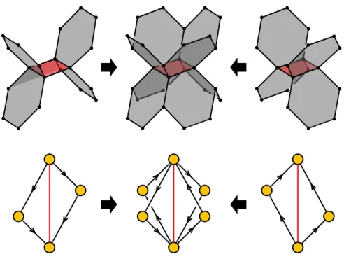
2d (0,2) theories are specified by the quiver, namely the gauge symmetry and matter content, and theJ- andE-terms for all Fermi fields. Remarkably, for theories corresponding to toric CY4, this information can be encapsulated in a single graphical object: theperiodic quiver. Periodic quivers were originally introduced in the context of abelian orbifolds of C4 in [3] and were later extended to generic toric singularities in [6].
A periodic quiver lives on a 3-torusT3 and is such that the individual contributions to J- andE-terms are encoded in terms of certainminimal plaquettes, as schematically shown in figure1.4 A plaquette is defined as a closed loop in the quiver consisting of an arbitrary
3Since all fields in the class of theories under study are bifundamental or adjoint, they are neutral under the diagonal combination of all nodes.
4What we precisely mean by “minimal” will be clarified in later sections, once we consider the dual of the periodic quiver.
JHEP02(2016)047
i Jji
Eij
j
i j
i j
i j
i j
Jji+
Jji Eij+
Eij
⇤ij
⇤ij
⇤ij
⇤ij
Figure 1. The four plaquettes (Λij, Jji±) and (Λij, Eij±) corresponding to a Fermi field Λij.
Y Z
D X
Figure 2. A unit cell of the periodic quiver of C4.
number of chiral fields and a single Fermi field. The chiral fields in a plaquette form an oriented path with two endpoints connected by the Fermi field, which closes the loop.
The toric condition (2.2) implies that for every Fermi field Λij there are four plaquettes (Λij, Eij±) and (Λij, Jji±), which share the undirected edge associated to Λij.
It is sometimes useful to visualize the periodic quiver as a tessellation of R3 by a unit cell. The simplest example of a periodic quiver corresponds to D1-branes over C4, for which the unit cell is shown in figure 2 [3]. All abelian orbifolds ofC4 can be constructed by combining copies of theC4 unit cell with periodicity conditions determined by the action of the generators of the orbifold group [3,6].
JHEP02(2016)047
1 2
1 1
1 1
1
1
2
2 2
2
2
2
quiver periodic quiver
Figure 3. The standard and periodic quivers for C ×C.
0 1 2 3 4 5 6 7 8 9
NS × × × × × × · · · ·
NS0 × × × × · · × × · · NS00 × × · · × × × × · ·
D4 × × × · × · × · · ·
Table 1. Brane configuration for brane box models. The (246) directions are compactified on aT3.
Figure 3 shows the periodic quiver for C ×C, where C indicates the conifold. Several additional examples of periodic quivers can be found in [6] and in the following sections.
2.2 Earlier constructions: brane box models for orbifolds
The construction of brane setups realizing 2d(0,2) theories was pioneered in [3] with the introduction of brane box models, which are reviewed in this section. Brane box models are Type IIA configurations consisting of three types of orthogonal NS5-branes: NS, NS0 and NS00-branes, which extend along the (012345), (012367) and (014567) directions, re- spectively. In addition, there are D4-branes spanning (01246). The (246) directions are compactified on a T3. The 2d gauge theories live on the two directions (01) common to all the branes. Each type of NS5-branes breaks SUSY by one half. The D4-branes break SUSY by an additional half leading, generically, to 2d (0,2). The NS5-branes divide T3 into cubic “boxes” within each of which there is a stack of Ni D4-branes, giving rise to a U(Ni) gauge group in the 2d theory. All branes sit at the same position in the (89) directions. The U(1) R-symmetry is given by the rotational symmetry in the (89) plane.
Table1 summarizes the brane configuration.
Brane box models are related to systems of D1-branes over abelian orbifolds of C4 by T-duality along (246) [3]. These configurations are natural generalizations of brane boxes with a single type of NS5-branes (also known as elliptic models), which correspond to the 6d theories associated to orbifolds of C2 [12], and brane boxes with two types of NS5-branes, which describe the 4dtheories for orbifolds of C3 [13,14].
JHEP02(2016)047
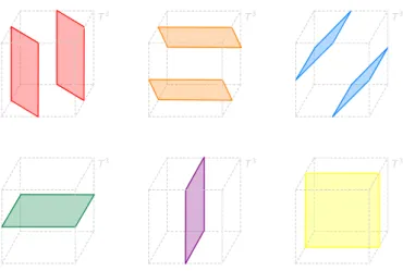
Figure 4. Brane box models. Schematic representation of the internal (2,4,6) directions. The blue, red and green planes correspond to NS, NS0 and NS00-branes that extend along (24), (26) and (46) directions. D4-branes span the (246) directions, filling the boxes. The geometric action of the dual abelian orbifold ofC4 is translated into the periodicity conditions on T3.
It is possible to place k NS, k0 NS0 and k00 NS00-branes such that they divide the T3 into kk0k00 boxes. Such a configuration is T-dual to a C4/(Zk×Zk0 ×Zk00) orbifold.
The geometric action of the orbifold is encoded in how the brane boxes are periodically identified. Figure4illustrates the basic features of a brane box model along the internalT3. There is a straightforward translation between brane box models and the corresponding periodic quivers mentioned in section2.1. The simplestC4 theory corresponds tok=k0 = k00 = 1 and hence has a single box. The theory has four chiral fields. Three of them define unit vectors in the T3: (1,0,0), (0,1,0), (0,0,1) and are hence transverse to the NS5-branes as illustrated in figure 5. We call them X, Y, Z, respectively. The fourth chiral field points in the (−1,−1,−1) direction. In the same basis, the three Fermi fields lie along the (0,1,1), (1,0,1), (1,1,0) directions, i.e. along the diagonals of the square faces of the box.
Brane box models have several positive features. First, they can be used to deduce the gauge theories associated to arbitrary abelian orbifolds of C4. In addition, they introduce the basic ingredients for brane configurations that are T-dual to D1-branes at toric singu- larities as well as some of their key characteristics such as their compactification on T3.
Despite all these successes, brane box models have several shortcomings. Overcoming them is one of the main goals of this paper. First of all, they do not provide the gauge theories for D1-branes on Calabi-Yau 4-folds beyond orbifolds. Furthermore, there is no one-to-one map between objects in the gauge theory and elements in the brane box model.
Most notably, while X, Y and Z-type chiral fields map to box faces, this is not true for D-type chiral fields. Similar arguments apply to the plaquettes involving these fields. In turn, this implies that basic symmetries of the gauge theories are not manifest in brane box models. Finally, brane box models do not relate to combinatorial objects that streamline their connection between CY4 geometry and gauge theory.
In the next section we introduce new constructions that overcome all these limitations.
In fact, brane box models can be regarded as degenerate limits of these more general setups.
JHEP02(2016)047
D Z Y X
Figure 5. Brane box models and periodic quivers. This figure presents the brane box model for C4, which has a single NS5-brane of each type. It also shows how the brane configuration gives rise to the corresponding periodic quiver. Orbifold models are obtained from this configuration by enlarging the unit cell.
3 Brane brick models
In this section, we introduce brane brick models, a novel class of brane configurations that provide a direct connection between toric Calabi-Yau 4-folds and the corresponding 2d (0,2) gauge theories. Brane brick models play a role analogous to the one of brane tilings, which correspond to 4d N = 1 gauge theories on D3-branes probing toric Calabi-Yau 3- folds. Not surprisingly, given the peculiarities of 2d (0,2) theories, brane brick models exhibit several original features as explained in the following sections.
3.1 Brane brick models as type IIA brane configurations
Brane brick models are Type IIA brane configurations that share basic features with brane box models [3]. They generalize the brane box construction to generic toric Calabi-Yau 4-folds that are not necessarily ofC4.
A brane brick model consists of an NS5-brane and D4-branes. The NS5-brane extends along the (01) directions and wraps a holomorphic surface (i.e. four real dimensions) em- bedded into the (234567) directions. The directions (246) are periodically identified to form a T3. It is therefore natural to pairwise combine (23), (45) and (67) into three complex variables x, y and z of which (246) are the arguments. The surface Σ wrapped by the NS5-brane is the zero locus of the Newton polynomial associated to the CY4,
X
(a,b,c)∈V
c(a,b,c)xaybzc = 0, (3.1)
where (x, y, z) take values in (C∗)3 and V is the set of points in the toric diagram on Z3. Stacks of D4-branes extend along (01) and are suspended within each of the voids cut
JHEP02(2016)047
Y Z X D
periodic quiver T3
Brane Brick
T3
Figure 6. The periodic quiver and dual brane brick modelT3 for theC4 theory.
out by the NS5-brane surface within the (246) 3-torus. Generically, the holomorphically embedded NS5-brane breaks 1/8 of the SUSY, while the D4-branes break an additional 1/2, resulting in a 2d(0,2) theory in the two common dimensions (01). As for brane boxes, the NS5-brane and the D4-branes sit at the same point in the transverse (89) dimensions and the U(1) R-symmetry of the gauge theory is geometrically realized as rotations on this plane.
From now on, we will primarily focus on a simpler object, which is obtained by replacing Σ by its skeleton or tropical limit. For simplicity, we will also refer to this object as the brane brick model. In this limit, Σ is replaced by a collection of 2dfaces that separate T3 into a collection of 3dpolytopes filled by D4-branes. We call the 3dpolytopesbricks.
3.2 The brane brick model — gauge theory dictionary
In section 2.1, we explained how the periodic quiver combines the quiver and J- and E-terms of a 2d (0,2) gauge theory into a single object. In analogy to the connection between brane tilings and periodic quivers for 4d N = 1 toric gauge theories [15], brane brick models can be constructed from the periodic quiver by graph dualization. Both constructions therefore contain precisely the same information. The dualization procedure forC4 is illustrated in figure 6.
The brane brick model for C4 contains a single brick, which corresponds to the only gauge group of the theory. This brick takes the form of a truncated octahedron consisting of eight hexagonal and four square faces, which correspond to chiral and Fermi fields, respectively.5 More generally, orbifolds ofC4are obtained by tessellatingT3with additional copies of the same type of brick. From now on, motivated by the convention for quivers, we will use black faces to indicate chiral fields and red ones to indicate Fermi fields. For C4, the faces of the brick are pairwise identified in T3 resulting, as expected, in four chiral fields and three Fermi fields in the adjoint representation of the gauge group. We can regard brane box models as degenerate limits of brane brick models forC4 and its orbifolds in which some faces shrink to zero size.
5Truncated octahedra have appeared in a similar context in [16].
JHEP02(2016)047
Brane Brick Model Gauge Theory
Brick Gauge group
Oriented face between bricks Chiral field in the bifundamental representation
iand j of nodesiand j (adjoint for i=j)
Unoriented square face between Fermi field in the bifundamental representation bricksiand j of nodesiand j (adjoint for i=j)
Edge Plaquette encoding a monomial in a
J- or E-term
Table 2. Dictionary between brane brick models and gauge theories.
Plaquettes in the periodic quiver correspond to edges in a brane brick model. The toric condition thus implies that Fermi fields correspond to squares. The converse is however not true and certain geometries lead to brane box models with square chiral faces. The four edges of a Fermi face split into two pairs, each of them contributing to a J- or E- term. For the C4 orbifold examples, one Fermi and two chiral faces meet at every edge.
This arrangement captures the structure of plaquettes in these theories and gives rise to the correspondingJ- and E-terms, all of which involve a pair of quadratic terms in chiral fields [3,6].
The basic dictionary between brane brick models and the corresponding gauge theories is summarized in table 2.
This article focuses only on topological properties of brane brick models. Whether there are preferred shapes for them and their significance is an interesting question that we postpone for further studies. A comparable example for brane tilings is given by isoradial embeddings and, in particular, the one encoding superconformal R-charges [17]. We now elaborate on some entries of the dictionary in further detail.
Chirality. Let us explain how brane brick models incorporate chirality, namely how to assign orientations to their faces. As usual, the orientation of a face can be translated into the orientation of its edges. By convention, if all edges in the perimeter of a face are oriented clockwise/counterclockwise, as seen from the interior of a brick, we say that it cor- responds to a chiral field in the dual periodic quiver pointing towards the exterior/interior of the brick.
The entire brane brick model can be systematically oriented as follows. We start from a face associated to a chiral field and assign to it the corresponding orientation. We then continue consistently orienting adjacent faces, whenever possible, until covering all edges.
At the end of this process, some square faces will turn out not to have a definite orientation.
These unoriented faces are precisely those that correspond to Fermi fields, which lack a notion of chirality. Figure 7 illustrates this procedure for C4. A more intrinsic algorithm for identifying unoriented faces corresponding to Fermi fields, which does not depend on the initial choice of a face associated to a chiral field, is presented in section 4.
Edges, plaquettes and Fermi fields. As previously mentioned, every edge in a brane brick model corresponds to a plaquette. Since every plaquette is associated to a Fermi
JHEP02(2016)047
Figure 7. Faces in a brane brick model can be systematically oriented starting from one associated to a chiral field. Faces corresponding to chiral fields are oriented while faces corresponding to Fermi fields are not.
Figure 8. The four plaquettes corresponding to a Fermi field face in brane brick models for C4 and its orbifolds.
field, we conclude that every edge is the boundary of at least one Fermi face. This is illustrated in figure 8, which shows the neighborhood of a Fermi face in the brane brick models for C4 and its orbifolds. While the faces associated to the initial and final chiral field in a plaquette must share the corresponding edge with the Fermi, intermediate chiral fields may not, as we now explain.6
It is possible for more than one Fermi face to be adjacent to the same edge. This is the case when the chiral fields in a plaquette are a subset of those in a larger plaquette.
This phenomenon occurs in Q1,1,1 for which a brane brick model will be studied in detail
6In the case of linear contributions toJ- orE-terms associated to chiral-Fermi massive pairs, the initial and final chiral field in the corresponding plaquette coincide.
JHEP02(2016)047
3 2
1
1 2
3 2
1
⇤421
⇤¯121 ¯⇤121
⇤421
¯⇤121·X24·D41 ⇤421·X12·X24·D41·D12
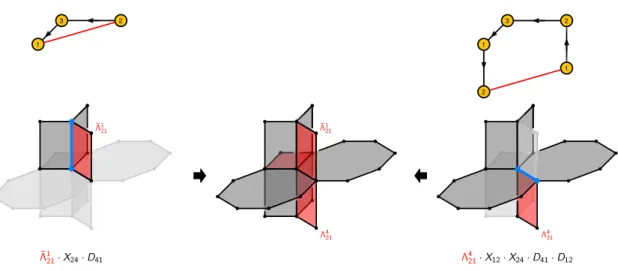
Figure 9. Two adjacent Fermi fields in the brane brick model for Q1,1,1 and two of the corre- sponding plaquettes. The chiral fields in the small plaquette are contained inside the second one.
in section 8.2.2. The J- and E-terms of this theory contain the following contributions J214−=X12·X24·D41·D12, E211− =X24·D41 . (3.2) We see that E211− ⊂ J214−. The corresponding plaquettes are shown in figure 9 and are associated to adjacent Fermi fields Λ421 and ¯Λ121.
To conclude this section, let us note that there are several ways of constructing brane brick models. First, they can be obtained by dualizing the periodic quiver, as explained in this section. In addition, they can be systematically obtained by partial resolution/higgsing from known ones, such as the ones forC4 orbifolds. Finally, it is possible to construct them directly from the probed geometry by means of a procedure which we call the fast inverse algorithm, as explained in section 4.
3.3 Mass terms and higgsing
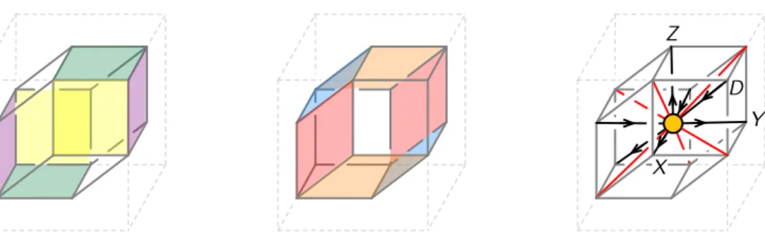
Higgsing. When a non-zero VEV is turned on for the scalar component of a bifunda- mental chiral field Xij, the gauge groups associated to quiver nodes i and j are higgsed to the diagonal subgroup. From the perspective of the brane brick model, this amounts to removing the face associated to Xij, which results in the combination of the bricks for nodesi and j into a single one, as schematically shown in figure 10. Deleting the face for Xij also has the desired effect of replacing it by its VEV, which without loss of generality is taken to be equal to 1, in all the plaquettes containing it.
Massive fields. Massive fields correspond to Fermi-chiral pairs extending between the same pair of gauge groups, such that either the J- or E-term for the Fermi field contains a term that is linear in the chiral field. In the brane brick model, these linear terms are represented by edges that are connected to a single Fermi face and a single chiral face. We refer to such edges as massive edges.
JHEP02(2016)047
Figure 10. Giving a non-zero VEV to a chiral field maps to deleting the corresponding face, here shown in blue, in the brane brick model. This results in the combination of two adjacent bricks into a single one.
... ...
... ...
fik(X) ⇤ki
Xij
Xjk
Jik=XijXjk fik(X) Jik=Xjk fik(X)
Xjk!fik(X)
a b
c d
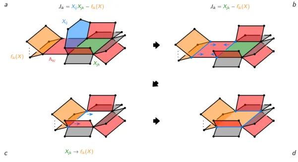
Figure 11. Generating a massive Fermi-chiral pair by higgsing and integrating it out. (a) Starting from Jik =XijXjk−fik(X), a VEV forXij generates a massive edge connecting Λki to Xjk, as shown in (b). (c) The massive edge and the opposite one in the face for Λki are merged, making the face disappear. (c) The replacementXjk →fik(X) removes the face forXjk and (d) glues its edges to the one forfik(X).
Massive fields can be generated in a variety of ways. Higgsing is one of them. In this case, a massive pair arises when an originally quadratic J- or E-term becomes linear after turning on a VEV. In the brane brick model, such terms correspond to edges that initially are attached to a Fermi and two chiral faces. When the face associated to the field acquiring the non-zero VEV is deleted, a massive edge is generated, as shown in figure 11(a).
As an example, let us consider a quadratic J-term for the Fermi field Λki that becomes linear when the chiral field Xij receives a VEV as follows7
Jik =XijXjk−fik(X) −→ Xjk−fik(X) . (3.3)
7The case of a linearE-term is identical.
JHEP02(2016)047
The gauge indices work properly, since nodesiandj are identified by the higgsing. Recall that all Fermi faces are squares. In (3.3),fij(X) indicates a product of chiral fields associ- ated with one of the edges attached to Λki. The linear term Xjk inJik corresponds to the opposite edge on the Λki face. This massive edge is indeed attached to the two massive fields: Λki and Xjk.
At low energies, Λki and Xjk can be integrated out. In this process, the termsJik and Eki associated to Λki are removed from the Lagrangian. This is nicely captured by the brane brick model as shown in figure 11, from steps (b) to (d). When integrating out the massive fields,Jik is set to zero and we replaceXjk →fik(X). For clarity, it is convenient to split this process into two stages, although no physical interpretation should be assigned to the intermediate step (c). The first step, shown in (c), corresponds to shrinking the face associated to Λki until the massive edge and the opposite one merge into a single one that we associate to fik(X). When doing so, the two other edges of Λki, which represent Eki, also disappear. Finally, in step (d), the face for Xjk is removed and the edges that formed its perimeter, with the exception of the massive edge, are glued to the one forfik(X). This implements the replacement Xjk →fik(X) in all J- andE-terms.
Let us conclude this section with a few additional remarks regarding the brane brick models obtained by integrating out massive fields. The procedure summarized in figure 11 faithfully incorporates all pertinent manipulations of the gauge theory. The two chiral faces shown in orange end up having three consecutive common edges. This might naively seem a little odd, since it may require curved brick faces. This, on its own, is not an issue at the level of discussion in the current paper, since we are only concerned with the combinatorial properties of brane brick models. More importantly, this feature can be simply avoided if the three edges are collinear or, as it occurs in several of the explicit examples we have studied, additional fields become simultaneously massive. In the latter case, integrating out all massive fields leads to configurations in which no pair of chiral faces is glued along three consecutive edges.
4 Brane brick models from geometry
This section studies the geometry of the brane brick model in further detail. This analysis will result in a new method for constructing the brane brick model directly from the underlying Calabi-Yau 4-fold. This procedure is a natural generalization of thefast inverse algorithm for brane tilings, which constructs the tiling from zig-zag paths [18,19]. We refer to the algorithm for brane brick models in the same way.
4.1 Amoebas and coamoebas
As explained in section 3.1, the NS5-brane in a brane brick model wraps a holomorphic surface Σ defined as the zero locus of the Newton polynomial of the toric CY4 cone.
Reproducing (3.1) here for convenience, Σ is hence defined by X
(a,b,c)∈V
c(a,b,c)xaybzc = 0. (4.1)
Σ is 2-complex dimensional, i.e. 4-real dimensional.
JHEP02(2016)047
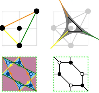
Figure 12. The toric diagram, the amoeba, a singular “approximation” to the coamoeba deter- mined by the zig-zag paths (shown in color) and the brane tiling for dP0.
Two natural projections help us to visualize and to study Σ. The first one, called the amoeba [20, 21], is a projection onto (log|x|,log|y|,log|z|) ∈ R3. The amoeba is a smooth geometric object dual to the toric diagram. The second projection, the coamoeba, maps Σ onto (arg(x),arg(y),arg(z)) ∈ T3. The coamoeba captures the geometry of the NS5-brane in the internal T3 and hence contains the non-trivial information necessary to define the corresponding quiver gauge theory. Both the amoeba and the coamoeba are 3-real dimensional objects. Visualizing them is challenging, but it is possible to get a flavor of their general structure by considering their analogues in the simple case of toric Calabi- Yau 3-folds with 2dtoric diagrams. Such objects have been studied in the physics context in [19] and figure12 presents a simple example.
We refer to the points at the corners of toric diagrams, both for Calabi-Yau 3-folds and 4-folds, as extremal points. In order to simplify our presentation, in the rest of the paper we assume that toric diagrams do not contain additional intermediate points on the edges connecting pairs of extremal points. All our ideas, however, extend to the general situation in which such points are present.
The example in figure 12 illustrates the general fact that for Calabi-Yau 3-folds the amoeba goes to infinity along “legs” that approach a linear behavior normal to the sides of the toric diagram. Similarly, in the Calabi-Yau 4-fold case the amoeba contains a leg for every edge of the 3dtoric diagram, along which it asymptotes to a plane normal to the edge under consideration. More concretely, for two extremal points in the toric diagram with coordinates (mx, my, mz) and (nx, ny, nz), the equation defining Σ simplifies to an equation consisting of only two terms
c(mx,my,mz)xmxymyzmz +c(nx,ny,nz)xnxynyznz = 0 (4.2)
JHEP02(2016)047
Figure 13. Toric diagram forC4.
when (some of) (|x|,|y|,|z|) go to infinity along the corresponding leg of the amoeba. In this limit, the amoeba projection of Σ becomes the 2dplane given by
(nx−mx, ny−my, nz−mz)·(log|x|,log|y|,log|y|) = 0, (4.3) up to a shift controlled by the values of the c(mx,my,mz) and c(nx,ny,nz) coefficients.
Similarly, the coamoeba simplifies considerably when approaching infinity along each leg of the amoeba, also becoming a 2d-plane orthogonal to the corresponding edge of the toric diagram, in this case living in T3. We refer to each of these planes as a phase boundary.8 Each phase boundary is thus controlled by a pair of extremal points in the toric diagram and given by
(nx−mx, ny−my, nz−mz)·(arg(x),arg(y),arg(z)) = 0. (4.4) Once again, each plane can be shifted by tuning the coefficients in the Newton polynomial.
In other words, phase boundaries are planes in T3 with winding numbers (nx−mx, ny− my, nz−mz). More generally, accounting for dual gauge theories sometimes requires de- forming phase boundaries while preserving their homology. This possibility will be explored in a forthcoming publication [22]. Phase boundaries are the brane brick model analogues of zig-zag paths in brane tilings.
The union of all phase boundaries contains a proxy for the boundary of the coamoeba, which gets replaced by a collection of planar facets. It is thus possible to discuss how phase boundaries divideT3 into two types of regions, corresponding to the interior and the complement of the coamoeba. In order to illustrate our previous discussion, let us consider theC4 example, for which the toric diagram is shown in figure 13. In this particular case, all coefficients in the Newton polynomial can be removed by rescalings and we have
1 +x+y+z= 0. (4.5)
Each of the six edges of the toric diagram in figure13gives rise to a phase boundary, as shown in figure14. Phase boundaries are presented in the same colors of the corresponding edges in the toric diagram.
8Here we use a nomenclature that is closer to the standard one in the mathematical literature. In a previous work [6], we referred to these objects as coamoeba boundaries or coamoeba planes.
JHEP02(2016)047
T3 T3 T3
T3 T3 T3
Figure 14. The six phase boundaries in T3 corresponding to the six edges of the toric diagram of C4. We use the same colors for the planes and their normal edges in figure13.
The six phase boundaries divide T3 into various regions, which correspond to either the interior or the complement of the coamoeba. In the example at hand, they carve out a singlerhombic dodecahedron (RD)9 in the complement, as shown in figure15.10
4.2 Periodic quivers from coamoebas
The periodic quiver, or equivalently the brane brick model, can be constructed from the phase boundaries of the corresponding Calabi-Yau 4-fold. In short, there is a node in the quiver for every component into which the phase boundaries split the complement of the coamoeba and chiral and Fermi fields arise at every point intersection of three or more phase boundaries.11 We refer to this procedure as the fast inverse algorithm for brane brick models. In the remainder of this section, we elaborate its detailed implementation.
Consider the C4 example as an illustration. The RD is identified with the single gauge group of the corresponding gauge theory, as shown in figure 15. We see that every point intersection of phase boundaries corresponds to a field in the periodic quiver. Equivalently, such intersections map to faces in the brane brick model, as illustrated in figure 16.
Let us now study how the orientability of phase boundary intersections allows us to distinguish between chiral and Fermi fields. We will illustrate the ideas in the context of theC4 example, but they straightforwardly generalize to more complicated Calabi-Yau 4- folds. In order to study the orientation of phase boundaries, which are objects living in 3d, it is useful to dissect the problem into a collection of 2dprojections. To do so, we consider
9Coamoeba and their phase boundaries onT3 have been studied in the mathematical literature [23].
10Stating that the RD is in the complement of the coamoeba requires a criterion for, starting from knowledge of the phase boundaries, identifying the complement of the coamoeba from its interior. In this simple example, we can take a shortcut by exploiting our knowledge of the periodic quiver, since by definition its nodes live in the complement of the coamoeba. Below we will introduce an algorithm for making this identification in generic theories.
11As for zig-zags in the case of brane tilings, phase boundaries need to be shifted inT3 until reaching a configuration that can be interpreted as consistent gauge theory.
JHEP02(2016)047
Y Z
D
X
Figure 15. C4 has six phase boundaries that cut out a RD in T3, which gives rise to the single gauge group of the corresponding gauge theory. The RD has eight 3-valent vertices and six 4-valent vertices that in this case are periodically identified in pairs and correspond to the four chiral and three Fermi fields of theC4theory, respectively.
brane brick
T3
coamoeba boundaries T3
Figure 16. Complement of the coamoeba cut out in T3 for C4 by the phase boundaries and the corresponding brane brick model. For convenience, the unit cell has been rotated with respect to the one used in figure15.
each of the faces of the toric diagram and assign an outward pointing normal vector to each of its edges, as shown in figures17 and 18.12
Every edge in the toric diagram is contained in a pair of faces and hence the previous prescription assigns to it a pair of vectors. By construction both vectors live on the plane orthogonal to the edge, i.e. on the corresponding phase boundary. We would now like to combine these vectors into a single one determining the orientation of the phase boundary.
For our purposes it is sufficient to take the sum of them.13 The resulting vector points towards the exterior of the toric diagram. Notice that this is an orientation on the phase boundary plane and not one orthogonal to it. There is no natural orientation normal to phase boundaries, since this would correspond to an inexistent orientation of edges in the toric diagram.
Phase boundaries divide the neighborhood of any point intersection into a collection of polyhedral cones. Depending on the behavior of the orientations of phase boundaries in these cones, we can distinguish two types of intersections, which we now explain.
12This is precisely the procedure for determining zig-zag paths associated to the external edges of 2dtoric diagrams in the case of Calabi-Yau 3-folds.
13Any linear combination of the two vectors with non-zero positive coefficients would also do the job.
JHEP02(2016)047
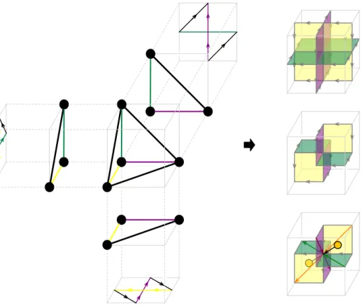
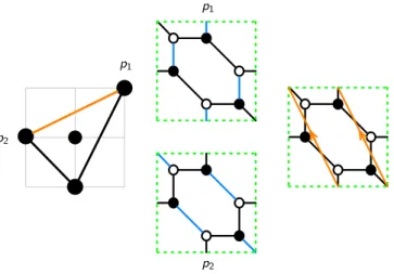
Figure 17. An oriented intersection between the three phase boundaries associated to the green, yellow and purple edges in the toric diagram ofC4. The pair of 2dfaces in the toric diagram that share a given edge determine the orientation of the corresponding phase boundary. Each projection gives rise to a collection of oriented lines on T2 that correspond to the intersection between the phase boundaries and a plane passing through the intersection. The chiral field extends along the oriented cones, connecting two gauge groups that live in the complement of the coamoeba.
Oriented intersections: chiral fields. We define anoriented intersection as one con- taining two oppositeoriented cones. An oriented cone is one for which all phase boundaries are oriented towards the point intersection or away from it. Notice that the number of phase boundaries participating in the oriented cones might be lower than the total number of phase boundaries in the intersection. Every oriented intersection gives rise to a chiral field, whose orientation is determined by the oriented cones.
Since matter fields in the quiver stretch between gauge groups, which in turn map to components in the complement of the coamoeba, the previous prescription also serves for distinguishing the interior from the complement of the coamoeba. From all the cones meeting an oriented intersection, only the oriented ones correspond to corners of regions in the complement of the coamoeba. Figure 17 illustrates the previous ideas for an oriented intersection in C4.14
14All examples considered in this section are such that for every pair of intersecting phase boundaries, the projections of their orientations onto their line intersection are parallel. This property is not generic.
Our general discussion applies even when this is not the case.
JHEP02(2016)047
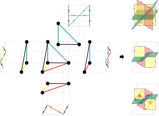
Figure 18. An alternating intersection between the four phase boundaries associated to the yellow, red, green and blue edges in the toric diagram of C4. The orientation of each phase boundary is established by considering the pair of 2dfaces in the toric diagram associated to it. The Fermi field extends along the two cones with alternating orientations, connecting two gauge groups that live in the complement of the coamoeba.
Alternating intersections: Fermi fields. Every alternating intersection contains a pair of special alternating cones. Alternating cones are such that the orientations of the line intersections between consecutive pairs of phase boundaries alternate between going into and away from the intersection. This implies that a necessary condition for a cone to be alternating is to involve an even number of phase boundaries. It is natural to conjecture that alternating cones always comprise four phase boundaries, an observation supported by all the explicit examples we have considered.
Every alternating intersection gives rise to a Fermi field, which extends along the two alternating cones. Similarly to the oriented intersection case, the corresponding pair of nodes in the quiver lay within the alternating cones, which can thus also be used to identify the complement of the coamoeba. Figure 18 shows an alternating intersection for C4 and the steps involved in determining the corresponding Fermi field.
To conclude this section, it is important to emphasize that the distinction between intersections leading to chiral and Fermi fields depends on their orientation or lack thereof and not on the number of intersecting phase boundaries. It is possible for a point intersec- tion of phase boundaries to be neither oriented nor alternating. When this occurs, it does not correspond to any field in the gauge theory.
JHEP02(2016)047
1 2 1 2
C C⇥C
Figure 19. Quiver diagrams for the 4dCtheory and for the 2dC ×Ctheory obtained from it by dimensional reduction.
5 Geometry from brane brick models
Brane brick models greatly simplify the determination of the probed toric Calabi-Yau 4-fold starting from the corresponding 2d (0,2) quiver gauge theories, providing an alternative to the forward algorithm studied in [6]. A similar feat is achieved by brane tilings, which connect 4dN = 1 gauge theories to Calabi-Yau 3-folds, and it is at the heart of some of their most important applications. This combinatorial approach is often referred to as the fast forward algorithm, and we will employ the same name for its 2danalogue. A crucial point for achieving this, which will be elaborated in this section, is a correspondence be- tween GLSM fields and certain objects in the brane brick model with simple combinatorial properties that we call brick matchings. They play a role analogous to perfect matchings for brane tilings.
In order to get some useful intuition for identifying what brick matchings are, it is convenient to review perfect matchings first. A perfect matching is a collection of edges in a brane tiling such that every node in the tiling is the endpoint of exactly one edge in the perfect matching. Every node in the tiling corresponds to a superpotential term in the 4d gauge theory or, equivalently, to a plaquette in the dual periodic quiver. We can thus alternatively define a perfect matching as a collection of chiral fields that contains exactly one field for every plaquette in the periodic quiver. An important property that follows from their definition is that all perfect matchings for a given brane tiling contain the same number of edges, which is equal to half the number of superpotential terms in the theory.15 Let us now move to the 2d case and try to find a combinatorial interpretation for GLSM fields. A natural starting point is theP-matrix, which relates chiral fields to GLSM fields. Several explicit examples can be found in [6].
For concreteness, let us consider the C ×Ctheory [6]. Its quiver diagram is shown in figure 19. TheJ- and E-terms are
J E
Λ112: X21·X12·Y21−Y21·X12·X21 = 0 Φ11·Y12−Y12·Φ22 = 0 Λ212: Y21·Y12·X21−X21·Y12·Y21 = 0 Φ11·X12−X12·Φ22 = 0 Λ121: X12·Y21·Y12−Y12·Y21·X12 = 0 Φ22·X21−X21·Φ11 = 0 Λ221: Y12·X21·X12−X12·X21·Y12 = 0 Φ22·Y21−Y21·Φ11 = 0
(5.1)
15This is not the case, however, for almost perfect matchings, which generalize perfect matchings to bipartite graphs with boundaries [24].
JHEP02(2016)047
The corresponding P-matrix is
P =
p1 p2 p3 p4 s X21 1 0 0 0 0 X12 0 1 0 0 0 Y21 0 0 1 0 0 Y12 0 0 0 1 0 Φ11 0 0 0 0 1 Φ22 0 0 0 0 1
. (5.2)
This simple example already exhibits a crucial difference between brick matchings and perfect matchings: brick matchings may involve different numbers of chiral fields. Here, everypi contains a single chiral field, while scontains two chiral fields.
5.1 Phase boundaries and brick matchings
As already discussed in section4, phase boundaries are analogous to zig-zag paths in brane tilings. In this section, we will generalize the well-known connection between perfect match- ings and zig-zag paths to a new relation between brick matchings and phase boundaries.
This will finally allow us to define brick matchings.
Perfect matchings are in one-to-one correspondence with GLSM fields for the 4dquiver theories associated to brane tilings and hence map to points in the 2d toric diagrams of the corresponding Calabi-Yau 3-folds [15,25]. We refer to the perfect matchings located at extremal points of the toric diagram asextremal perfect matchings. Perfect matchings can be endowed with an orientation, e.g. by orienting all edges from white to black nodes. The zig-zag path associated to an external edge in the toric diagram corresponds to the differ- ence between the two extremal perfect matchings connected by the edge [26]. Figure 20 illustrates the construction of zig-zag paths from extremal perfect matchings for the dP0 example.
We can think about phase boundaries as collections of faces on the brane brick model, as shown in figure 21 for C4. It is useful to introduce the phase boundary matrix H to encode this information. Columns in this matrix correspond to phase boundaries ηα and rows correspond to chiral and Fermi fields, i.e. to faces in the brane brick model. An entry in Hiα is equal to ±1 if the face associated to the row i is contained in the boundary represented by the column α (with the sign controlled by the relative orientation) and 0
JHEP02(2016)047
p1
p2
p1
p2
Figure 20. The toric diagram and brane tiling for dP0. The figure illustrates the construction of a zig-zag path (orange) as the difference of the two extremal perfect matchings p1 andp2.
otherwise. For C ×C, we have
H=
η12 η23 η34 η41 η1s η2s η3s η4s
X12 1 −1 0 0 0 −1 0 0 X21 −1 0 0 1 −1 0 0 0 Y12 0 0 1 −1 0 0 0 −1 Y21 0 1 −1 0 0 0 −1 0
Φ11 0 0 0 0 1 1 1 1
Φ22 0 0 0 0 1 1 1 1
Λ112 0 0 1 −1 1 1 1 0
Λ212 1 −1 0 0 1 0 1 1
Λ121 −1 0 0 1 0 1 1 1
Λ221 0 1 −1 0 1 1 0 1
. (5.3)
We can also regard H as summarizing the net intersection numbers, counted with orienta- tion, between the phase boundaries and the fields in the periodic quiver within a unit cell.
Our goal is to establish a one-to-one correspondence between brick matchings and GLSM fields. This, in turn, will determine that brick matchings are mapped to points in the 3d toric diagram of the underlying Calabi-Yau 4-fold. We expect brick matchings to correspond to collections of fields in the quiver and hence to collections of faces in the brane brick model. In analogy with the brane tiling case, it is natural to envisage that the phase boundary associated to an edge in the toric diagram is given by the difference between the two extremal brick matchings connected by the edge, i.e. ηµν =pµ−pν. It then becomes clear that if brick matchings consisted only of chiral fields, then the resulting surfaces would have holes corresponding to the Fermi fields. We conclude that brick matching must contain both chiral and Fermi fields.
Based on this reasoning, let us generalize theP-matrix to include Fermi fields. Allowing only for 1 and 0 entries depending on whether a brick matching contains a field or not, (5.3)
JHEP02(2016)047
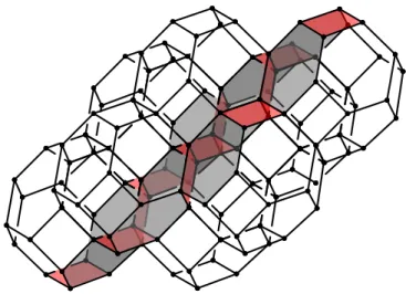
Figure 21. The brane brick model for C4 with a collection of highlighted chiral and Fermi faces that form one of its phase boundaries.
uniquely determines
PΛ=
p1 p2 p3 p4 s X12 0 1 0 0 0 X21 1 0 0 0 0 Y12 0 0 0 1 0 Y21 0 0 1 0 0 Φ11 0 0 0 0 1 Φ22 0 0 0 0 1 Λ112 0 0 0 1 1 Λ212 0 1 0 0 1 Λ121 1 0 0 0 1 Λ221 0 0 1 0 1
. (5.4)
The columns inPΛ do not correspond to the brick matchings we are after, yet.
Physically, Fermi fields Λa and their conjugate ¯Λaare on an equal footing. It is hence reasonable to consider a definition of brick matchings that treats them symmetrically. We thus also include rows for ¯Λain a newP-matrix, to which we refer asPΛ ¯Λ. This new matrix contains exactly the same information as PΛ. The entries for the ¯Λa rows are determined such that they obey
PΛ ¯Λ,Λaµ+PΛ ¯Λ,Λ¯aµ= 1. (5.5) It will soon become clear that this choice also leads to brick matchings with nice combina- torial properties. It is important to emphasize, though, that Λaand ¯Λa do not correspond to independent degrees of freedom.