JHEP05(2016)020
Published for SISSA by Springer
Received: March 3, 2016 Accepted: April 7, 2016 Published: May 4, 2016
Brane brick models and 2d (0, 2) triality
Sebasti´an Franco,a,b Sangmin Leec,d,e,f and Rak-Kyeong Seongg
aPhysics Department, The City College of the CUNY, 160 Convent Avenue, New York, NY 10031, U.S.A.
bThe Graduate School and University Center, The City University of New York, 365 Fifth Avenue, New York NY 10016, U.S.A.
cCenter for Theoretical Physics, Seoul National University, Seoul 08826, Korea
dDepartment of Physics and Astronomy, Seoul National University, Seoul 08826, Korea
eCollege of Liberal Studies, Seoul National University, Seoul 08826, Korea
fSchool of Natural Sciences, Institute for Advanced Study, Princeton, NJ 08540, U.S.A.
gSchool of Physics, Korea Institute for Advanced Study, Seoul 02455, Korea
E-mail: [email protected],[email protected], [email protected]
Abstract: We provide a brane realization of 2d (0,2) Gadde-Gukov-Putrov triality in terms of brane brick models. These are Type IIA brane configurations that are T-dual to D1-branes over singular toric Calabi-Yau 4-folds. Triality translates into a local trans- formation of brane brick models, whose simplest representative is a cube move. We present explicit examples and construct their triality networks. We also argue that the classical mesonic moduli space of brane brick model theories, which corresponds to the probed Calabi-Yau 4-fold, is invariant under triality. Finally, we discuss triality in terms of phase boundaries, which play a central role in connecting Calabi-Yau 4-folds to brane brick models.
Keywords: Brane Dynamics in Gauge Theories, D-branes, Supersymmetric gauge theory ArXiv ePrint: 1602.01834
JHEP05(2016)020
Contents
1 Introduction 1
2 Brane brick models 3
3 2d (0,2) SQCD and triality 6
4 Triality for brane brick models 9
4.1 Triality and brane brick models 11
4.2 Transformation ofJ- and E-terms 13
5 Examples 15
5.1 Triality network for Q1,1,1 15
5.2 Triality network for Q1,1,1/Z2 19
6 The mesonic moduli space 19
6.1 The fast forward algorithm 20
6.2 A detailed example 22
6.3 General invariance of the mesonic moduli space 24
6.4 Connection to (2,2) duality 25
7 Triality and phase boundaries 25
7.1 Phase boundaries for cubic nodes 25
7.2 Phase boundaries under triality 28
7.3 Phase boundaries as collection of faces 30
7.4 Possible connections to integrable systems 32
8 Conclusions 32
A Phases of Q1,1,1 34
B Phases of Q1,1,1/Z2 41
1 Introduction
While 2d N = (0,2) theories have only two supercharges, their dynamics is under con- siderable control due to chirality, holomorphy and anomalies. In recent years, we have witnessed remarkable developments in our understanding of these theories. They include:
c-extremization [1, 2], exact CFT description of the low energy limit of SQCD-like theo- ries [3], detailed studies of renormalization group (RG) flows [4], connections to 4dN = 1
JHEP05(2016)020
theories via dimensional reduction [5, 6] and to 6d (2,0) theories by compactification on 4-manifolds [7]. In addition, it has been discovered that 2d(0,2) theories exhibit IR du- alities [8] similar to Seiberg duality in 4d N = 1 gauge theories [9]. This low energy equivalence is calledtriality, since it is only after three of these transformations acting on the same gauge group that we return to the original theory.
Embedding quantum field theories in string or M-theory provides a powerful grip on their dynamics. This approach has been particularly helpful for understanding, and in some cases uncovering, quantum field theory dualities in various dimensions and with different amounts of supersymmetry. This program has been recently extended to 2d(0,2) gauge theories, following the pioneering work in [10]. In [11], a systematic procedure for deriving the 2d(0,2) gauge theories on the worldvolume of D1-branes probing generic singular toric Calabi-Yau (CY) 4-folds was developed.1 The general structure of this infinite class of the- ories was then studied in detail. The brane engineering of these gauge theories was taken a further step forward in [15], which introduced a new type of Type IIA brane configurations, denotedbrane brick models, which are related to the D1-branes over toric CY4singularities by T-duality. Brane brick models fully encode the gauge theories on the worldvolume of the D1-branes and extremely simplify the connection to the probed geometries.
The previous discussion leads to a natural question: is there a brane realization of 2d (0,2) triality? This is the central topic we set to explore in this article, in which we will explain how triality is nicely realized in the context of brane brick models.
In this article we will see that, in general, brane brick models associate a class of 2d (0,2) quiver gauge theories to every toric CY4 singularity. The multiple gauge theories within a class can be constructed using several methods developed in [11, 15]. They turn out to be related by triality, which is realized as a local transformation of the brane brick models.2 The simplest example of this transformation is a cube move. The probed CY4
corresponds to the mesonic moduli space of the gauge theories and it is thus common to all brane brick models related by triality. As shown in [3, 4], 2d (0,2) SQCD theories with different ranks of the three flavor groups exhibit triality as an exact IR equivalence even when the classical mesonic moduli spaces are different. Our brane brick models are, however, similar to the case of SQCD with equal ranks of the flavor groups, for which the three phases share the same moduli space.
This paper is organized as follows. Section 2 reviews the basic concepts of the brane brick models introduced in [15]. Section 3 reviews the original proposal of [8] for triality for 2d (0,2) supersymmetric QCD and certain quiver generalizations. Section 4 explains how triality is implemented in terms of brane brick models. Section 5 presents explicit examples, for which we construct part of their triality networks [8]. In section 6, we show in examples that triality preserves the classical mesonic moduli space and sketch a general
1Other interesting recent approaches for constructing 2d (0,2) theories include: stacks of D5-branes wrapped over 4-cycles of resolved/deformed conifolds fibered over a 2-torus [12], compactifications on Rie- mann surfaces of 4d N = 1 quiver gauge theories on D3-branes over CY3 singularities [13] and F-theory compactifications on singular, elliptically fibered CY 5-folds [14].
2In a sense, the situation is reminiscent of the early investigations oftoric duality [16,17]. Several 4d N = 1 gauge theories were constructed for a given toric CY3 singularity. It was later realized that the transformation relating different theories associated to the same CY3was precisely Seiberg duality [18,19].
JHEP05(2016)020
0 1 2 3 4 5 6 7 8 9
D4 × × × · × · × · · ·
NS5 × × ———– Σ ———— · ·
Table 1. Brane brick models are Type IIA configurations with D4-branes suspended from an NS5-brane that wraps a holomorphic surface Σ.
proof of its invariance for general brane brick models. In section 7, we examine triality from the perspective of phase boundaries, which bridge CY4 singularities and brane brick models. Section8offers conclusions and directions for future work. In the two appendices, we collect detailed data for the explicit examples used in the main text.
2 Brane brick models
This section contains a lightning review of brane brick models. Its primary goal is to introduce the basic concepts and nomenclature. It is not intended to be complete, and we encourage the reader to look at [11,15] for in depth presentations.
Brane brick models were introduced in [15] as a powerful tool for studying the 2d (0,2) quiver gauge theories that arise on the worldvolume of D1-branes probing toric CY4 singularities. A brane brick model is a Type IIA brane configuration of D4-branes sus- pended from an NS5-brane. The NS5-brane extends along the (01) directions and wraps a holomorphic surface (i.e. four real dimensions) Σ embedded into the (234567) directions.
The directions (246) are periodically identified to form a T3. The coordinates (23), (45) and (67) are pairwise combined to form three complex variables x,y and zof which (246) are the arguments. The surface Σ is given by the zero locus of the Newton polynomial associated to the toric diagram of the CY4: P(x, y, z) = 0. Stacks of D4-branes extend along (01) and are suspended inside the voids cut out by Σ on the T3 given by the (246) directions. The 2d(0,2) gauge theory lives in the (01) directions, which are common to all the branes. Table 1summarizes the basic ingredients of a brane brick model.
Most of the non-trivial information concerning a brane brick model is captured by its skeleton on theT3. For brevity, we will refer to both the full brane configuration and this simpler object as the brane brick model. Every brane brick model fully encodes a 2d(0,2) gauge theory according to the dictionary in table 2. Bricks correspond to U(N) gauge groups.3 There are two types of faces. First, there are oriented faces, which correspond to chiral fields. In addition, there are unoriented faces, each of which represents a Fermi field Λ and its conjugate ¯Λ. Fermi faces are always 4-sided. Finally, edges of the brane brick model are associated to monomials in J- or E-terms. For detailed discussions of 2d (0,2) theories, including their supermultiplet structure and the construction of their Lagrangians in (0,2) superspace, we refer to [5,8,10,20].
Brane brick models are in one-to-one correspondence with periodic quivers on T3. Periodic quivers also fully capture the gauge symmetry, matter content, and J- and E-
3All ranks are equal in the T-dual of a stack of regular D1-branes at the CY4. More generally, allowing for fractional D1-branes can lead to brane brick models in which bricks have different numbers of D4-branes.
JHEP05(2016)020
Brane Brick Model Gauge Theory
Brick Gauge group
Oriented face between bricks Chiral field in the bifundamental representation i andj of nodes iandj (adjoint fori=j)
Unoriented square face between Fermi field in the bifundamental representation bricks iandj of nodes iandj (adjoint fori=j)
Edge Plaquette encoding a monomial in a
J- orE-term
Table 2. Dictionary between brane brick models and 2dgauge theories.
i Jji
Eij
j
i j
i j
i j
i j
Jji+
J−ji Eij+
Eij−
Λij
Λij
Λij
Λij
Figure 1. The four plaquettes (Λij, Jji±) and (Λij, E±ij) associated to a Fermi field Λij. The J- andE-terms areJji=Jji+−Jji− = 0 andEij =Eij+−E−ij = 0, respectively, where Jji± andEij± are holomorphic monomials in chiral fields.
terms of a 2d(0,2) theory [11]. The latter correspond to minimal plaquettes. A plaquette is a closed loop in the quiver consisting of an oriented path of chiral fields and a single Fermi field. Every Fermi field in this class of theories is associated to two pairs of minimal plaquettes as shown in figure1, which translates into monomial relations from vanishing J- and E-terms. This is known as thetoric condition and is a general property of the gauge theories on D1-branes over toric CY4 singularities [11].
The brane brick model can be regarded as a tropical limit of the coamoeba projection of Σ onto (arg(x),arg(y),arg(z)).4 The alternative projection of Σ onto (|x|,|y|,|z|) is called theamoeba projection. The amoeba approaches infinity along “legs” that are in one- to-one correspondence with edges of the toric diagram. Along each of these asymptotic legs, the coamoeba simplifies and reduces to a 2d-plane in T3 that is orthogonal to the corresponding edge of the toric diagram. We refer to these planes asphase boundaries. We point the reader to [15] for the details of this construction.5
4For this reason, in the restricted context of orbifolds ofC4, this object has been referred to as atropical coamoeba[21].
5More generally, phase boundaries are 2d surfaces, not necessarily planes, whose homology on T3 is determined by the corresponding edge in the toric diagram [15].
JHEP05(2016)020
chiral
Fermi
Figure 2. Phase boundaries are in one-to-one correspondence with edges of the toric diagram of the Calabi-Yau 4-fold. Certain point intersections of phase boundaries give rise to chiral or Fermi fields, depending on whether they are oriented or alternating.
Brane brick models can be reconstructed from phase boundaries. This procedure is called thefast inverse algorithm and makes it possible to go from toric diagrams to brane brick models [15]. Chiral and Fermi fields arise at point intersections between them. Phase boundaries divide the neighborhood of every intersection point into a collection of cones.
In [15], we introduced a prescription for assigning an orientation to every phase boundary.
The distinction between chiral and Fermi fields depends on the orientation properties of the cones at the corresponding intersection. Chiral field are associated tooriented intersections, which are defined as those containing two opposite oriented cones. An oriented cone is one for which all phase boundaries on its boundary, which might be a subset of all the ones participating in the intersection, are oriented towards the intersection or away from it. On the other hand, Fermi fields correspond to alternating intersections, which are those that contain a pair of alternating cones. Alternating cones are cones in which the orientations of the line intersections between consecutive pairs of phase boundaries alternate between going into and away from the intersection. The chiral and Fermi fields in the periodic quiver associated to the two types of intersections are aligned with the corresponding oriented and alternating cones, respectively. Figure 2 presents two examples of this construction. It is possible for a point intersection of phase boundaries to be neither oriented nor alternating.
In this case, it does not correspond to any field in the gauge theory.
Remarkably, brane brick models not only encapsulate the entire 2d(0,2) gauge theory data, but also substantially simplify the connection to the probed CY4 geometry. We have already seen glimpses of this beautiful relation in our discussion of the interplay between toric diagrams, phase boundaries and brane brick models. The connection to geometry becomes even more tantalizing in terms of a new type of combinatorial objects denoted brick matchings. A brick matching is defined as a collection of chiral, Fermi and conjugate Fermi fields that contribute exactly once to every plaquette in the theory, while satisfying
JHEP05(2016)020
SU(2)
SU(Nb) SU(Nf) SU(2Nc−Nb+Nf)
Φ Ψ P Γ Ω
U(Nc) ⇤ ⇤ ⇤ · det SU(Nf) · ⇤ · · · SU(Nb) ⇤ · · ⇤ · SU(2Nc+Nf−Nb) · · ⇤ ⇤ · SU(2) · · · · ⇤
U(Nc)
Φ Ψ
P Γ
Ω
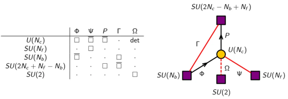
Figure 3. The quiver diagram for 2d(0,2) SQCD (original theoryD). Square nodes indicate flavor symmetry groups.
some additional simple rules (see section6.1for the complete definition). Brick matchings are in one-to-one correspondence with the GLSM fields describing the classical mesonic moduli space of the gauge theory, namely the CY4singularity. They are the key ingredients of the fast forward algorithm, a powerful method for obtaining the probed geometry [15], which we review in section 6.1.
3 2d (0,2) SQCD and triality
In this section, we review triality for 2d (0,2) theories. This is a low energy equivalence between gauge theories originally introduced in [8].
Let us consider 2d (0,2) SQCD with U(Nc) gauge group. This theory has Nb chiral fields Φ in the fundamental representation of U(Nc) and Nf Fermi fields Ψ in the antifun- damental representation. The Φ contribute 12Nb, the Ψ contribute −12Nf and the vector multiplet contributes −Nc to the SU(Nc)2 anomaly. The resulting −12(2Nc +Nb −Nf) anomaly can be cancelled by introducing 2Nc+Nb−Nf chiral multiplets P in the anti- fundamental representation of U(Nc). These three types of fields give rise to an SU(Nb)× SU(Nf)×SU(2Nc+Nb−Nf) global symmetry. In addition, we introduce a Fermi field Γ, which is a singlet of the gauge symmetry and transforms in the bifundamental representa- tion of the global SU(Nb)×SU(2Nc+Nb−Nf). Finally, in order to cancel the anomaly in the U(1) part of U(Nc), we introduce two Fermi multiplets Ω in the determinant representa- tion of U(Nc). The theory can be represented by the quiver diagram shown in figure3.6 We include a J-term for the Fermi field Γ: JΓ= ΦP. This term corresponds to the triangular plaquette in the quiver and is also sometimes referred to as a ΦPΓ superpotential.
Triality turns the original theory into the one shown in figure 4. The new gauge group is U(Nc0), with Nc0 =Nb−Nc. The structure of the new theory is identical to the original one up to a counterclockwise 120◦ rotation. This means that the fundamental chirals Φ, antifundamental chirals P and fundamental Fermis Ψ are replaced by antifundamental chiralsP0, fundamental Fermis Ψ0 and fundamental chirals Φ0, respectively. Borrowing the
6In this article we adopt the convention that the head and tail of the arrow associated to a chiral field correspond to fundamental and antifundamental representations, respectively.
JHEP05(2016)020
Φ0 Ψ0 P0 Γ0 Ω0 U(Nb−Nc) ⇤ ⇤ ⇤ · det
SU(Nf) ⇤ · · ⇤ · SU(Nb) · · ⇤ ⇤ · SU(2Nc+Nf −Nb) · ⇤ · · ·
SU(2) · · · · ⇤
U(Nb−Nc)
SU(Nf) SU(Nb)
SU(2Nc+Nf −Nb)
Γ0 P0 Φ0
Ψ0 Ω0
SU(2)
Figure 4. The quiver diagram for the dual of 2d(0,2) SQCD (dual theory D0).
terminology of 4dSeiberg duality, these fields are the analogues of magnetic flavors. This theory also requires a pair of Fermi fields Ω0 in the determinant representation of U(Nc0) to cancel the U(1)2 anomaly. The new Fermi singlet Γ0 is a mesonic field that, in terms of the electric flavors, is given by Γ0 = ΦΨ. The dual flavors and the Fermi meson are coupled by a superpotential Φ0P0Γ0. The disappearance of the original Fermi singlet Γ can be understood as follows. The original chiral fields combine into a chiral field meson M = ΦP in the dual theory, which transforms in the bifundamental representation of SU(2Nc+Nb−Nf)×SU(Nb). The original superpotential becomes MΓ, giving a mass for M and Γ, which can thus be integrated out and disappear at low energies.
Let us call the original theory in figure 3 theory D and the dual theory in figure 4 theory D0. Applying the triality transformation once more, we obtain a third theory D00. Its gauge group is U(Nc00), with Nc00 = Nb0 −Nc0 = Nf −Nb +Nc. As before, its quiver diagram is obtained from the one for D0 by a counterclockwise 120◦ rotation. It is only after a third dualization that we obtainNc000 =Nb00−Nc00=Nc and we return to the original theory. The fact that this is an IR equivalence between three theories motivates calling it a triality.
Relabeling the ranks of the flavor symmetry groups as N1 ≡2Nc−Nb+Nf,N2≡Nb
andN3 ≡Nf, the rank of the gauge group becomes Ni+N2j−Nk and the triality chain can be thought of as a cyclic permutation ofN1,N2 andN3. This is shown in figure5. From now on we omit the Fermi fields in the determinant representation of the gauge group. They are absent if the gauge group is SU(Nc) instead of U(Nc), since they are not required for anomaly cancellation. While the theories on D1-branes we will study have U(Nc) gauge groups, such fields are not required because abelian anomalies are cancelled by a generalized Green-Schwarz mechanism via interactions with bulk RR fields [22].
Substantial evidence for triality in 2d(0,2) SQCD was presented in [8] by matching the flavor symmetry anomalies, central charges, and the equivariant indices. Furthermore, an exact CFT description of the low energy physics of SQCD was given in [3] and an exact beta function for the K¨ahler modulus was determined in [4].
Triality for quiver gauge theories. In [8], triality was generalized to a special class of quiver gauge theories with multiple gauge and flavor nodes. In this class of theories, all chiral and Fermi fields are in bifundamental representations, aside from possible Ω Fermi
JHEP05(2016)020
N1 N1
N1
N2 N2
N2
N3 N3
N3
N1+N2−N3
2
N2+N3−N1
2
N3+N1−N2
2 P
P0
P00 Φ
Φ0
Φ00 Ψ
Ψ0
Ψ00 Γ
Γ0
Γ00
Figure 5. The triality loop for 2d(0,2) SQCD.
multiplets in determinant representations for cancellation of U(1)2 anomalies. Further- more, only J-terms are non-trivial. They are all quadratic, namely they come from cubic plaquettes, and every chiral field participates in at least one of them.
The transformation of such a theory under triality can be summarized as follows.
Consider acting on gauge node k. All other nodes in the quiver remain unaltered, while the rank of nodek becomes
Nk0 =X
j6=k
nχjkNj−Nk, (3.1)
wherenχjk is the number of chiral fields from node j to node k.
The field content around node kis modified according to the following rules:
(1) Replace each of (→k), (←k), (— k) by (←k), (— k), (→k), respectively.
(2) For each subquiveri→k→j, add a new chiral fieldi→j.
(3) For each subquiveri→k— j, add a new Fermi fieldi— j.
(4) Remove all chiral-Fermi pairs generated in the previous steps.
(3.2)
The fields generated at steps 2 and 3 can be regarded as composites of those in the original theory. We will thus often refer to them as mesonic fields.
Later in this paper we will extend triality to the class of theories associated to brane brick models. In particular, such theories can have a richer structure of J- andE-terms.
JHEP05(2016)020
Triality networks and triality loops. Acting with triality on all the gauge groups of a quiver generates a family of IR equivalent gauge theories that can be neatly organized into atriality network [8]. Triality networks can contain triality loops, namely closed sequences of triality transformations that return to the original theory. The simplest example of a triality loop, which is present in every theory, is the triangular loop associated to three consecutive triality transformations on the same gauge group. Figure 5 shows the triality loop for 2d(0,2) SQCD.
Chiral conjugation. We define chiral conjugation as a global operation on a quiver that reverses the directions of all chiral fields and exchangesJ- andE-terms. Let us denote the local triality at node k by τk and chiral conjugation by γ. Clearly, τk3 = 1 and γ2 = 1.
Upon inspection of the transformation rule (3.2), we note thatτk and γ satisfy
γτkγ =τk−1 =τk2. (3.3)
As a result, the triality loop associated to three consecutive triality transformations on the same gauge group of the chiral conjugate configuration is isomorphic to the original one, except that the orientation of the loop is reversed.
4 Triality for brane brick models
The goal of this section is to introduce a triality proposal for brane brick models. We will not consider triality transformations of arbitrary gauge groups. Instead, we will focus on those such that the resulting gauge theories are also described by brane brick models. We refer to such theories as toric phases. In order to shape our proposal, we will combine a natural generalization of the basic triality transformation with various desired properties for the resulting theories.
Ranks. Let us first consider the ranks of gauge groups. Toric phases associated to N regular D1-branes on a toric CY 4-fold must have all ranks equal to N.7 What types of nodes can in principle be dualized such that, the resulting rank remains equal to N? It is reasonable to assume that the transformation rule for ranks of the basic triality continues to apply for these more general theories. Specializing (3.1) to a node k in a toric phase, we get
Nk0 =nχk,inN −N . (4.1)
In order to obtain Nk0 = N we need nχk,in = 2, i.e. nodes with only two ingoing chiral field arrows.
The cancellation of non-abelian anomalies further constraints the dualized node. As discussed in [11,15], the cancellation of SU(Nk)2 anomalies requires that
X
j6=k
(nχjkNj+nχkjNj−nFkjNj) + 2(aχk −aFk)Nk= 2Nk. (4.2)
7Notice that dual phases with unequal ranks might exist, as we briefly mention in section 3. Such theories, however, are not described by brane brick models.
JHEP05(2016)020
Figure 6. General configuration for a node in the periodic quiver whose dualization leads to another toric phase. The example we show corresponds to nχk,out=nFk = 4.
When all gauge nodes have equal ranks, the relation simplifies to
nχk−nFk = 2. (4.3)
Combining (4.2) withnχk,in= 2, we conclude that the dualized node must have
nχk,out =nFk . (4.4)
Summarizing what we have learnt so far: in order to remain within toric phases, we have to dualize nodes with nχk,in = 2 and nχk,out =nFk ≥2. The lower bound follows from the fact that, in order to avoid SUSY breaking in this class of theories, both nχk,in and nχk,out must be greater or equal than 2.
The Quiver. Let us now consider the transformation of the quiver. We also assume that the fields charged under the dualized node and the new mesons obey the rules in (3.2). In order for the dual theory to correspond to a brane brick model, we should not generate mesons that correspond to lines crossing over the dualized node or interlaced loops of fields in the periodic quiver. A natural solution to this problem is given by a local configuration of the general form shown in figure 6 for the case ofnχk,out=nFk = 4
The orientations of chiral fields in this configuration are such that, as illustrated in figure 7, the dual theory does not have mesons going over the dualized node or interlaced loops. Furthermore, we chose the outgoing chiral fields and the Fermi fields to alternate along an equatorial plane. This alternation facilitates the construction of plaquettes, and hence it is a natural structure to arise in toric theories.8
Plaquettes. So far, we have only explained how the quiver transforms under a triality transformation. A full definition of triality for toric phases also requires a rule for obtaining the J- and E-terms in the dual theory. We propose the following prescription for doing so: after performing the local transformation of the dualized node shown in figure 7, the J- andE-terms are those that follow from the resulting periodic quiver. This prescription will be illustrated in numerous examples in section 5, for which the J- and E-terms are explicitly presented in the two appendices.
8It would be interesting to determine whether more general configurations are possible.
JHEP05(2016)020
Figure 7. Local transformation of the quiver under triality for a node with nχk,out=nFk = 4. The initial configuration is such that the dual is also a toric phase, i.e. it continues to be well described by a periodic quiver.
As reviewed in section 3, a triality prescription for a wide class of quiver theories was introduced in [8]. Our proposal applies to a different class of quiver gauge theories, hence considerably extending the range of applicability of triality. Our theories have more general J-terms, non-trivial E-terms and are engineered in terms of branes.
Loops of toric phases and cubic nodes. Following our previous discussion, starting from a toric phase and dualizing any node of the general form shown in figure 6 with nχk,in = 2 and nχk,out = nFk ≥ 2, we obtain a new toric phase. According to the rules in (3.2), nχ0k,in in the dual theory is equal to nFk of the original one. Hence, a second dualization on the same node will result in a toric phase only if nFk = 2. This implies that nodes with nχk,in = nχk,out = nFk = 2 are not just the simplest configurations that can be dualized to obtain a toric phase. They are also special because it is only for them that the triality loops of three consecutive dualizations on the same node exclusively involve toric phases. The corresponding bricks in the brane brick models have six faces, as shown on the left of figure 9. We thus refer to these nodes as cubic nodes.
For the aforementioned reasons, most of our discussion in coming sections will focus on triality of cubic nodes. An explicit example of a toric phase obtained by a triality transformation of a node with nχk,in>2 will be discussed in section 5.1.
4.1 Triality and brane brick models
We now rephrase our previous discussion from the viewpoint of brane brick models, focusing on triality transformations of cubic nodes.
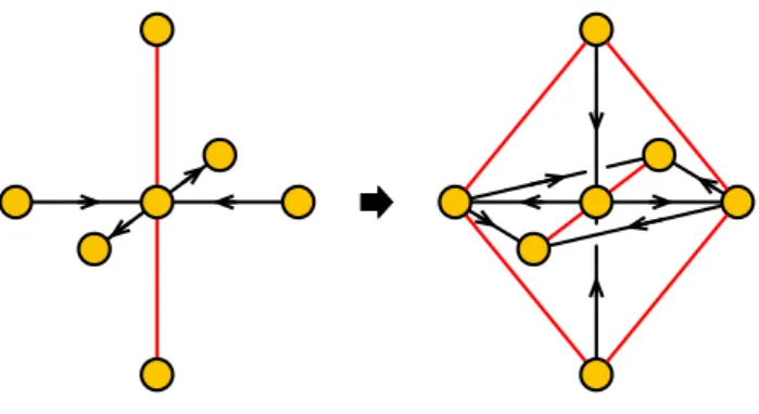
A cubic node has six nearest neighbors. For simplicity, let us begin by assuming that, before the triality move, there are no fields connecting the nearest neighbors among themselves. The triality move on the cubic node is shown in figure 8.
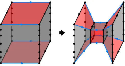
Translating figure 8 into a brane brick model by the usual graph dual method, we arrive at figure9. As explained in [15], it is convenient to keep track of the orientation of brick faces by assigning orientations to their edges.
Recall that Fermi faces are always quadrilaterals. Chiral faces are less restricted. We will not assume that the chiral faces of the cube before triality are necessarily simple
JHEP05(2016)020
Figure 8. Local triality action on a cubic node in the periodic quiver.
Figure 9. Local triality action on a cubic brick.
squares, by which we mean four sided. Instead, we will allow the common boundary between two chiral faces to carry a sequence of oriented edges. Figure 9 shows examples of composite boundaries containing three vertical edges.
Under these conditions, the local brick configuration after triality is determined uniquely as shown on the right of figure 9. The original cube is replaced by a new, smaller, cube consisting of chirals and Fermis determined by the triality rule. In addition, eight new “diagonal” faces are produced, which connect a subset of the edges of the original cube to edges in the new cube. The edges are oriented such that four of the diagonal faces are Fermis and the other four are chirals. Note that, in order for the diagonal mesonic chiral faces to have even number of edges, the number of edges constituting the composite boundary in the initial cube should be odd.
Faces associated to fields that are neutral under the dualized gauge group may undergo modifications. Consider the blue edges of the cubic brick shown in figure 9. Unlike the other eight edges in the cube, they are not connected to new mesonic faces in the dual theory. Faces outside of the cube that are initially attached to the blue edges remain connected to them. In the process, each of them gains two new edges as shown in figure9.
If a face glued to such an edge was a (2k)-gon before triality, it would become a (2k+2)-gon
JHEP05(2016)020
Figure 10. Integrating out a massive chiral-Fermi pair in a brane brick model.
afterwards. This is perfectly fine for a chiral face, but seems problematic for a Fermi face.
Interestingly, the apparent problem occurs if and only if the periodic quiver containsnested plaquettes. Nested plaquettes refer to the case in which the chiral fields in a plaquette are a subset of those in a larger plaquette (see [15] for a discussion). In the brane brick model perspective, nested plaquettes arise when more than one Fermi faces share a common edge.
Establishing how to modify figure 9 in the presence of nested plaquettes would require a more refined analysis. In all examples considered in this article, this phenomenon arises only when we dualize a node that leads to a toric phase but that it is not cubic. Since we will mainly focus on triality moves on cubes, we will not delve into the subtleties associated to nested plaquettes.
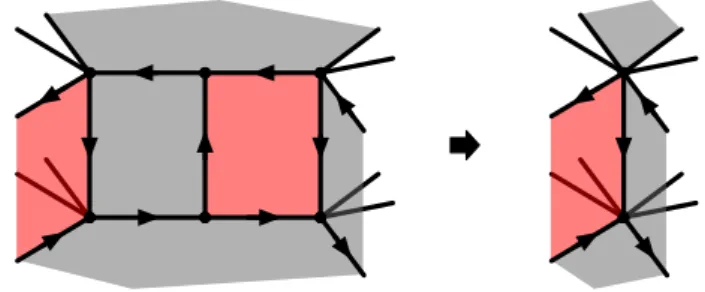
Triality can also give rise to chiral-Fermi massive pairs. As explained in [15], such a pair corresponds to a Fermi and a chiral faces connected by an edge to which no other face is attached. Massive pairs can be integrated out at low energies, simplifying the brane brick model. This process is illustrated in figure 10.
All the discussion in this section also applies if we relax our initial assumption on the absence of fields running between the six nearest neighbors. Moreover, in all the explicit examples considered in the next section, these pre-exiting fields form massive pairs with mesonic fields and disappear at low energies.
4.2 Transformation of J- and E-terms
2d(0,2) theories must satisfy the vanishing trace condition X
a
tr (JaEa) = 0. (4.5)
In [11], partial resolution was used to show that all brane brick models satisfy this condition.
Here we would like to take a complementary approach to this problem. We will show that, for brane brick models, triality preserves the vanishing trace condition.
We find it convenient to introduce a formal object for bookkeeping J- and E-terms,
Ω =X
a
tr ΛaJa+ ¯ΛaEa
. (4.6)
Using a formal inner product, (Λa)ij·( ¯Λb)kl=δbaδilδjk, wherei, j, k, lare (anti)fundamental indices at appropriate gauge nodes, we can rewrite the vanishing trace condition as
Ω·Ω =X
a
tr (JaEa) = 0. (4.7)
JHEP05(2016)020
4
2
0 5
3
6 1
4
2
0 5
3
6 1
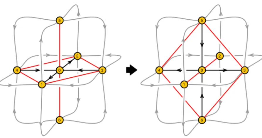
Figure 11. Transformation ofJ- andE-terms. The curved grey arrows represent oriented chains of chiral fields.
For simplicity, let us begin with the local triality move shown in figure 11. In the figure, we included open chains of chiral fields connecting pairs of adjacent neighbors to the cubic node. We denote them byOij.
Let us assume that the plaquettes near the cubic nodes are simply those we can rec- ognize in figure 11. The formal sum Ω before the triality is
Ω = Ω0+ Λ13(X30X01−O31) + Λ31(O15O53−O16O63) + Λ14(X40X01−O41)−Λ41(O15O54−O16O64) + Λ23(X30X02−O32)−Λ32(O25O53−O26O63) + Λ24(X40X02−O42) + Λ42(O25O54−O26O64) + Λ05(O53X30−O54X40)−Λ50(X01O15−X02O25) + Λ06(O63X30−O64X40) + Λ60(X01O16−X02O26).
(4.8)
Here, Ω0 collects the contributions from plaquettes whose Fermi fields are not shown in the figure. We suppressed the “tr” symbol, but the cyclic ordering in a monomial should be understood. We also suppressed the bar from ¯Λ, with the identification Λji = ¯Λij.
A simplifying feature of the local quiver in figure11is that the tr(EaJa) terms involving the four chiral and six Fermi fields shown explicitly cancel among themselves, leaving
Ω·Ω = Ω0·Ω0−(O31O15O53) + (O25O53O32+O41O15O54+O63O31O16)
−(O16O64O41+O32O26O63+O54O42O25) +O42O26O64. (4.9) For the theory to be consistent, this sum should vanish.
In the local quiver of figure11, the triality acts as a cyclic permutation on node labels:
(123456)→(345612). But, theOijOjkOklterms in (4.9) are grouped in cyclically invariant combinations. So, if Ω·Ω vanishes before triality, it should still vanish after the triality.
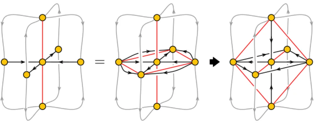
There are local quiver configurations that look more complicated than figure 11. For example, at first sight, the left quiver in figure8does not seem to allow for an augmentation by external chains of chiral fields Oij with obvious assignments of plaquettes. Fortunately,
JHEP05(2016)020
=
Figure 12. Massive chiral-Fermi pairs added to the initial configuration in figure 8 so that the transformation rule of figure11can be applied directly.
by integrating in/out chiral-Fermi pairs, we can bring an arbitrary local quiver into the simple form of figure 11. As an illustration, applying this idea to figure 8, we arrive at figure 12.
5 Examples
In this section we investigate some explicit examples. As mentioned earlier, we primarily focus on triality acting on cubic nodes. In order to do so, it is necessary to find toric CY 4-folds that give rise to brane brick models containing cubic bricks. Fortunately, a theory of this type was already identified in earlier work [11, 15]. It corresponds to D1-branes probing the cone over Q1,1,1. In order to generate an additional example with a richer triality structure, we will simply consider the Q1,1,1/Z2 orbifold. Following the general construction for orbifolds of toric geometries introduced in [11,15], a brane brick model for this orbifold is obtained by taking one for Q1,1,1 and appropriately doubling the size of the unit cell. Figure 13 shows the toric diagrams for both geometries.
To keep our discussion succinct, we will mostly phrase it in terms of periodic quivers.
The brane brick models for all the theories studied in this section are presented in the appendices, which collect additional detailed information about these theories, such as explicit expressions for theirJ- and E-terms.
5.1 Triality network for Q1,1,1
Let us start from the periodic quiver shown in figure 14. This theory was introduced in [11, 15], where it was shown that it corresponds to D1-branes probing the cone over Q1,1,1. We will refer to it as theasymmetric phase (A), since it is not manifestly invariant under the octahedral symmetry permuting the three axes. This is indeed a symmetry of the underlying geometry, as it follows from the toric diagram.
The brane brick model for this theory is presented in appendix A. The periodic quiver contains two types of nodes. Nodes 1 and 2 correspond to cubic bricks, while nodes 3 and 4, to octagonal cylinders.
JHEP05(2016)020
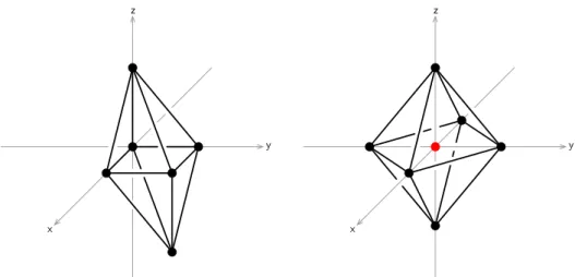
x
y z
x
y z
Figure 13. The toric diagrams forQ1,1,1 (left) andQ1,1,1/Z2 (right).
4
3
2 4
1
3 1
2 1
3 2 4
4 1 3
1
4 2
4
3 1
2 1
2
1
1 3
x
y z
Figure 14. Periodic quiver for phase A ofQ1,1,1. Notice that the region represented has twice the volume of the unit cell.
Let us consider the action of triality on a cubic node, say 1. The resulting theory is identical to the original one up to a cyclic permutation of the three axes. Figure 15shows the triality loop arising from three consecutive dualizations of node 1.
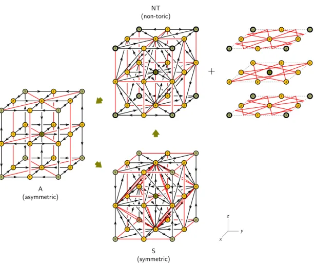
Let us now consider what happens when dualizing node 3. Interestingly, while this node is not cubic, it is of the general form discussed in section 4 and shown in figure 7.
We thus know that triality on it takes phase A to another toric phase. The new theory is shown at the bottom right of figure 16. It is indeed a toric phase and, furthermore, it is invariant under the permutation of the coordinate axes. We hence refer to it as the symmetric phase (S).9 It is important to note that in this periodic quiver, the multiplicity of the Fermi lines that are adjoints of node 4 is two. This special feature follows from how
9It is interesting to remark that phase S can also be directly determined from theQ1,1,1geometry using the general methods introduced in [11,15], without reference to triality.
JHEP05(2016)020
4
3
2 4
1
3 1
2 1
3 2 4
4 1 3
1
4 2
4
3 1
2 1
2
1
1 3
4
3
2 4
1 3
2 1
3 1
4 2
1
3 2 4
4 1 4
3 1
2 1
2
1
1 3
4
3
2 4
1 3
2 1
3 1
4 2
1
3 2 4
4 1 4
3 1
2 1
2
1
1 3
x y z
Figure 15. Action of three consecutive triality transformations on the cubic node 1 of phase A of Q1,1,1. It simply amounts to a cyclic permutation of the threeT3directions.
the periodic quiver capturesJ- andE-terms for this theory, is related to details of its brane brick model and is discussed in detail in appendix A.
Continuing with a second dualization on node 3 generates a non-toric phase (NT), which we show at the top right of figure 16. The rank of node 3 in this theory is 3N. Since the theory is non-toric, it is not fully captured by a periodic quiver, i.e. there is no known prescription for reading the J- and E-terms directly from it. The quiver diagram in figure 16 should be understood merely as a representation of the gauge symmetry and matter content of the theory. A third dualization on node 3 returns to the toric phase A.
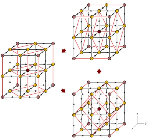
Figure 16 shows the triangular loop obtained by three consecutive dualizations on node 3. In order to place the dualized node at the center, we have shifted the periodic quivers with respect to figure14 by half a period in thex direction. It is straightforward to verify that the three theories are free of non-abelian anomalies, which is in fact guaranteed by the triality transformation rules.
We can combine our previous analyses to construct a piece of the triality network for Q1,1,1 involving only dualizations on nodes 1 and 3. The result is shown in figure 17 and consists of the triality loop in figure 15 and three permutations of the triality loop in figure 16. Since phase S is invariant under the permutation of coordinate axes, it sits at the intersection of the triality loops of all the three versions of phase A.
JHEP05(2016)020
1
x y z A
(asymmetric)
4
3 1
2
3 4
4 2
1
2 1 3
3 1 3
4
2 2
4
3 1
2
3 4
3 1 3
2
1
4 2
3
1 3
4 3
1 4 2
2 3 3
2 4
1 3
4
3
4 2
1
4 2
3
1 3
4 3
1 4 2
2 3 1
3
2 4
2
1 3
4 3
3
3 1
4
2
1 3
4 3
2
3 1 3
1
4 2
3 1
4
2
4 4
2
1 3
4 3
2
3 1 3
+
S (symmetric)
NT (non-toric)
3 1 3
2
Figure 16. Action of three consecutive triality transformations on the node 3 of phase A of Q1,1,1. The symmetric phase S is a new toric phase. Notice that in this periodic quiver the Fermi lines attached to node 4 are double. The U(3N) gauge node in phase NT is distinguished by a thick boundary.
A A
A
S NT
NT NT
Figure 17. A piece of the triality network forQ1,1,1, involving only dualizations of nodes 1 and 3.
JHEP05(2016)020
4
3
7 5
1
6 8
2 8
3 7 4
4 8 6
8
4 2
5
6 8
7 8
7
8
8 6
x
y z
Figure 18. Periodic quiver for phase A ofQ1,1,1/Z2.
The brane brick model for phase A contains another cube (node 2) and another octag- onal cylinder (node 4). Their behavior under triality is identical to the cases we considered, up to chiral conjugation. Of course, we may also perform triality moves on other nodes of phases S and NT, generating even more non-toric phases. We will not pursue them in this paper.
5.2 Triality network for Q1,1,1/Z2
We now perform a similar study for Q1,1,1/Z2. Our starting point is the theory defined by the periodic quiver in figure 18. Since it is simply related to figure14 by doubling the size of the unit cell, we also refer to it as phase A.
For simplicity, we will only consider triality acting on cubic nodes. Even with this restriction, the triality network has a much richer structure of toric phases than the one forQ1,1,1 due to the larger number of gauge groups.10
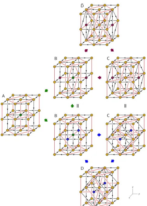
In order to simplify the presentation of results, we will identify theories that differ by a relabeling of the nodes in their periodic quivers. Restricting to theories connected to phase A by a sequence of dualizations on cubic nodes, the triality network for Q1,1,1/Z2 contains five distinct phases: A, B, C, D, ¯D. As the notation suggests, phases A, B, C are self-conjugate under chiral conjugation, whereas D and ¯D are conjugate to each other.
These theories form three minimal triality loops: (A-B-B), (B-C-D), (B- ¯D-C). Figure 19 shows a brief summary of the network and figure 20 provides further details. Detailed information regarding all these phases, including their brane brick models, is presented in appendix B.
6 The mesonic moduli space
In this section we will see that triality on brane brick models preserves their classical mesonic moduli space. This moduli space is the toric CY4 transverse to the probe D1-
10As forQ1,1,1, additional toric phases can be generated by dualizing certain non-cubic nodes. For brevity, we will not discuss such theories.
JHEP05(2016)020
B C
D D ¯ A
Figure 19. A piece of the triality network for Q1,1,1/Z2 containing phase A and restricting to dualizing cubic nodes. Theories differing by node relabeling are identified.
branes. A more interesting perspective on this fact is as follows. Brane brick models assign 2d (0,2) gauge theories to toric CY4 singularities. In general, a toric CY4 does not give rise to a single gauge theory, but to a class of them. Remarkably, at least for the large class of explicit examples we have considered, all theories within this class are in fact related by triality.11 It would be interesting to find a general proof of this statement, if it is indeed true as evidence suggests.
The mesonic moduli space can be computed using the forward algorithm developed in [11]. This calculation is in principle a straightforward exercise. However, it becomes extremely demanding already for theories such as the Q1,1,1/Z2 phases discussed earlier.
These complications are overcome by the fast forward algorithm, which was introduced in [15] and we summarize below.
6.1 The fast forward algorithm
We now briefly review the fast forward algorithm. Its key ingredients are the so-called brick matchings. Brick matchings are in one-to-one correspondence with GLSM fields in the toric description of the CY4 singularity. A crucial feature that makes them extremely powerful is that they are defined combinatorially. To do so, it is useful to completeJa- and Ea-terms into pairs of plaquettes by multiplying them by the corresponding Λa or ¯Λa. A brick matching is then defined as a collection of chiral, Fermi and conjugate Fermi fields that contribute to every plaquette exactly once as follows:
1. For every Fermi field pair (Λa,Λ¯a), the chiral fields in the brick matching covereither each of the two Ja-term plaquettes or each of the two Ea-term plaquettes exactly once.
2. If the chiral fields in the brick matching cover the plaquettes associated to the Ja- term, then ¯Λa is included in the brick matching.
3. If the chiral fields in the brick matching cover the plaquettes associated to the Ea- term, then Λa is included in the brick matching.
11When the 2dtheories have (2,2) SUSY, they are actually related by the (2,2) duality of [23], instead of triality.
JHEP05(2016)020
4
3
7 5
1
6 8
2 8
3 7 4
4 8 6 8
4 2
5
6 8
7 8
7
8
8 6
4
3
7 5
1
6 8
2 8
3 7 4
4 8 6 8
4 2
6 8
7 8
8
8
5 6
7 4
3
7 5
1
6 8
2 8
3 7 4
4 8 6 8
4 2
6 8
7 8
8
8
5 6
7
4
3
7 5
1
6 8
2 8
3 7 4
4 8 6 8
4 2
6 8
7 8
8
8
5 6
7
4
3
7 5
1
6 8
2 8
3 7 4
4 8 6 8
4 2
6 8
7 8
8
8
5 6
7 4
3
7 5
1
6 8
2 8
3 7 4
4 8 6 8
4 2
6 8
7 8
8
8
5 6
7
4
3
7 5
1
6 8
2 8
3 7 4
4 8 6 8
4 2
6 8
7 8
8
8
5 6
7
= =
A
B
B
D
C C D¯
x y z
Figure 20. A detailed version of the triality network for Q1,1,1/Z2 shown in figure 19. On each triality loop, the node on which the triality operates is given a different color.
The position of every brick matching in the toric diagram is determined by the inter- sections between the chiral field faces in the brick matching and the edges of the unit cell of the brane brick model, γa (a=x, y, z). The integer-valued coordinates, (nx, ny, nz)∈Z3, of a brick matching pare given by
na(p) = X
Xij∈p
hXij, γai, (6.1)
a=x, y, z, where the angle brackets indicate the standard intersection number between an orientated surface and an oriented line, contributing ±1 or 0 to the overall coordinate na.