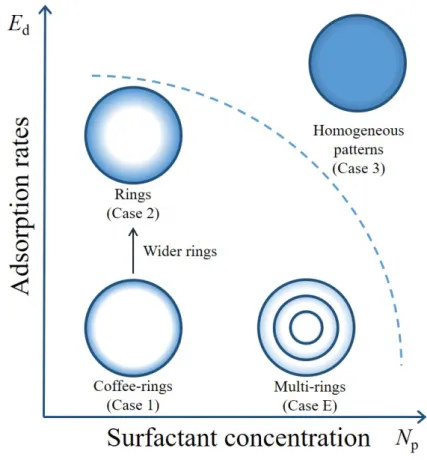
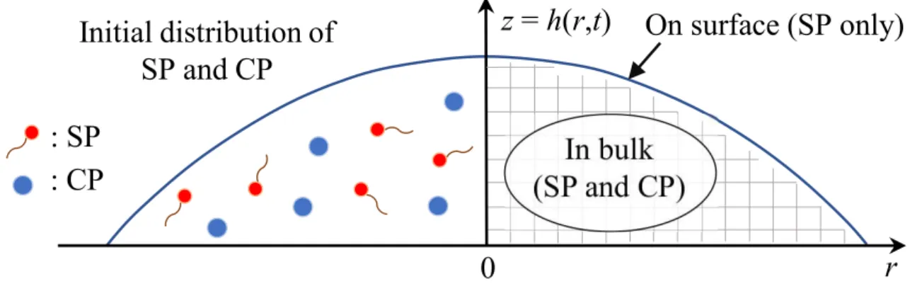
For slow adsorption rates, surfactant molecules are recirculated with the colloidal particles and the surface area covered by the surfactant grows from the contact line to the bulk of the droplet as the initial surfactant concentration increases. Marangoni currents can also develop inward through surfactant concentration gradients on the surface.
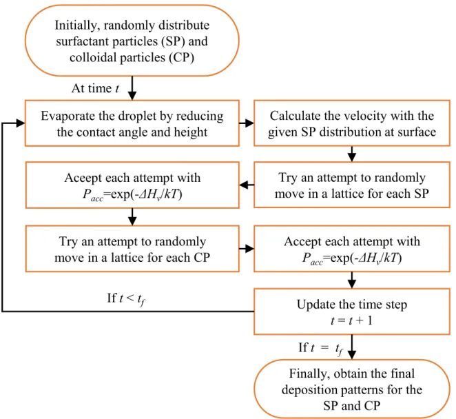
Monte-Carlo method for evaporation process of
The details of the mathematical formulation for this model and the Monte-Carlo method algorithm are described in Chapter II. These two studies were performed by developing a Monte Carlo approach based on the 2D Ising model proposed by Rabani et al.
Lattice Boltzmann method for evaporation process of droplet
Marangoni flows can also develop internally from surfactant concentration gradients at the surface, because the surface concentration increases with radius due to convection caused by external evaporation. In the presence of surfactant, the dynamics of colloidal particles changes dramatically due to the coupling of capillary flow and surfactant-induced flow at the droplet surface.
Model
- Langmuir’s isotherm for sorption kinetics
- Velocity field with non-zero Marangoni flow
- A coarse-grained lattice model
- Configurational Hamiltonian
- Evolution by the Monte Carlo method
To calculate g(r, t), we introduce the nonlinear surface equation of state for the surface tension s from the Langmuir isotherm model [21]. However, in a desiccation drop, the bulk surfactant is mainly transported to the subsurface by convection, which significantly reduces the surfactant absorption delay to the surface compared to diffusion.
Surfactant effects on droplet dynamics and deposition patterns
Effects of surfactant on dried patterns
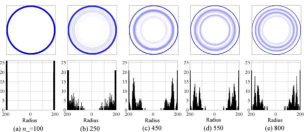
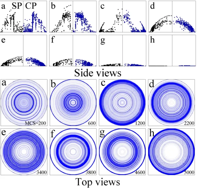
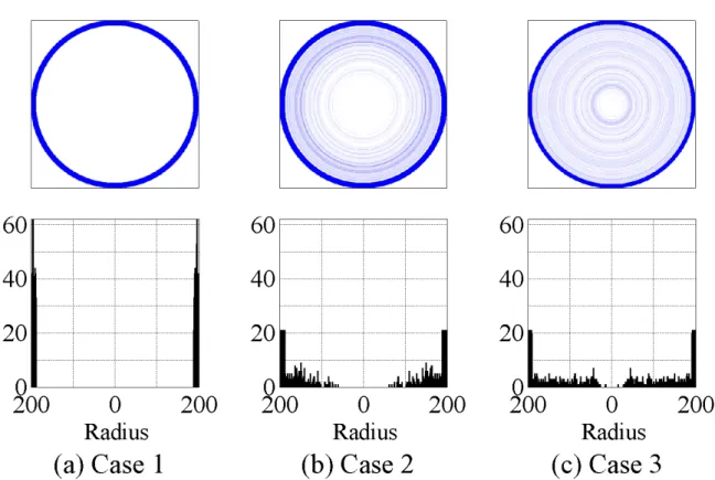
The effect of the parameter Q on the deposited patterns is studied by the simulations with and without surfactant. 2.3(a) shows a typical ring-shaped deposition pattern (the ring in blue at the contact line in the top view and bars in black in the side view), which ensures the ability of the present model to reproduce coffee ring patterns without wetting agent. As NSP increases, the width of the outer ring increases (from case A to B), after which multirings develop (for cases C–E).
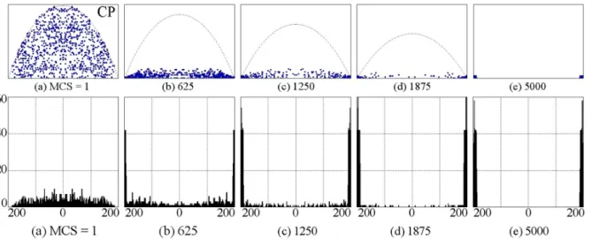
The final multi-ring pattern is quite different from the more uniformly distributed pattern of case 3, shown in Figure. It is also observed that the central regions of the deposits in cases B–E do not contain CP, which is mainly attributed to enhanced outward convection during the final phase of evaporation.
Effects of surfactant on flow patterns
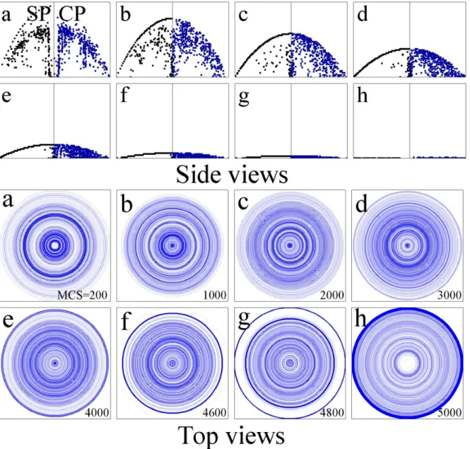
The dynamics of CP shows unique oscillatory motions at the contact line due to the coupling between the surfactant and droplet dynamics. At the same time, Marangoni flows are reduced due to the smaller aggregation of SP at the edge compared to regime (d). As a result of the SP sheet, inward Marangoni flow develops, and the coffee ring effect at the edge and the subsequent contact line dynamics of CP are significantly suppressed (Fig.
Due to the higher number of SPs adsorbed on the surface compared to case 2, stronger Marangoni currents are induced. This corresponds to the back and forth motion of the CP on the contact line shown in Fig.
Conclusions
Oscillation dynamics of colloidal particles caused by surfactant in an evap-
Particle dynamics and flow patterns
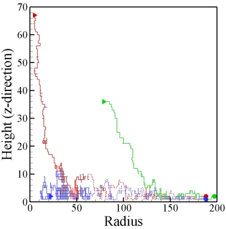
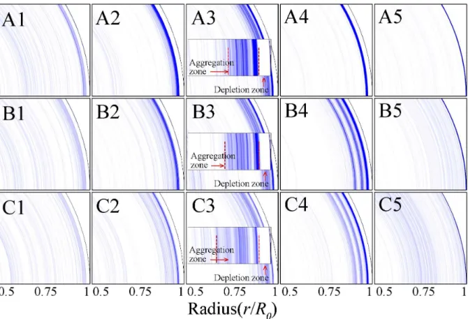
For case B and C with larger NSPs, the formation of accumulation and depletion zones during the early phase of evaporation also occurs as in case A. This verifies the occurrence of SP-induced Marangoni external flow at the droplet edge. It is of interest to note that the location of the accumulation zone is determined by the relative strength of the Marangoni outflow.
The velocity profiles for each model identify that the accumulation zone is formed at the inner end of the region dominated by the outer Marangoni flow. Therefore, the strength of the internal and external Ma flows is proportional to SP.
Time-dependent oscillatory movement of particles
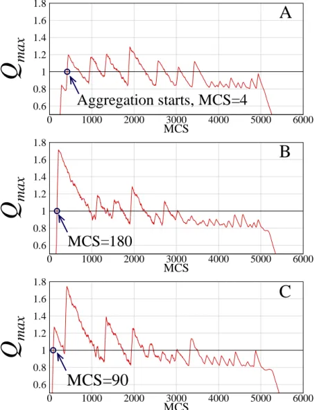
During the early stage of the evaporation (see Fig. 2.17a), the appearance of the aggregation and depletion zones is determined by the early formation of the coffee ring and the subsequent development of the Ma flow. Since the supply of SP to the coffee ring is greatly reduced by the outer Ma flow, the strength of the flow is maintained for a certain period of time. As the evaporation continues, the intensity of the coffee ring effect increases significantly over time.
For the same reason, in case A, aggregation and depletion zones develop in the early phase of evaporation (see Fig. 2.18a). At the same time, the temporal evolution of the external current Ma follows the mechanism in Figure 1b.
Conclusions
Since this phenomenon is undesirable in many industrial fields, such as coating [80], nanoassembly [81], nanopatterning [82] and inkjet printing [2], strategies are needed to control the deposition patterns based on the understanding of the evaporation mechanisms. of points and the deposition process. 45] clarified that the outward capillary flow is attributed to the coffee ring effect of the droplet. Due to such limitations of experimental study, many studies are trying to obtain the flow field either numerically or analytically.
For numerical studies, Zhao and Yong [84] developed a multiphase lattice Boltzmann model based on free energy to simulate the evaporation of a colloidal droplet on a solid surface with certain wetting properties. Our model consists of a pseudopotential LB model for droplet evaporation and an advection-diffusion LB model for colloids.
Model
- The lattice Boltzmann method
- The pseudopotential model
- A forced advection-diffusion equation
- Chapman-Enskog analysis
To include the interaction force in LBM, Shan and Chen [23] introduced the equilibrium velocity ukeq:. where ubulk is the macroscopic velocity of the bulk liquid:. Therefore, the macroscopic fluid velocity, Uf, which expresses the motion of the fluid, is defined by means of momenta before and after the collision step:. where ρ is the sum of densities of each component. Note that before solving the advection-diffusion equation of particle concentration, the lattice Boltzmann equation for the medium fluid is solved separately to obtain the velocity field of the fluid.
The distinguishing feature of the LB method for the advection-diffusion equation compared to the Navier-Stokes equation is that veqi is obtained externally from the velocity of the medium fluid (solvent), Uf, in Eq. Since the external force is applied to the colloidal particles at the interface of the medium fluid, the macroscopic velocity of the colloidal particle, v, is assumed to be changed, and can be obtained from Eq.
Results and discussions
Velocity field inside a pure droplet during evaporation
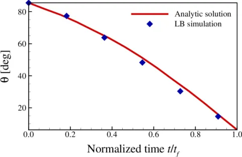
Thus, an equation describing the evolution of the point contact angle with constant contact radius mode can be derived as [11],. To quantitatively compare the flow field with the analytical solution, we plot the radial and vertical velocities corresponding to the drop height [35]. The solid line shows the analytical solution obtained from eq 3.28 and the symbols correspond to the LB simulation results. a) Line and (b) vector field of the flow field for the right half of the point.
The initial conditions of the drop are set as follows: the contact radius is R0 = 100 with the contact angle θ0 '90◦, and the densities. The initial density of the colloid particles is C = 0.5 inside the droplet, and the density outside the droplet is C = 0.01.
Conclusions
In the CFD community, the characteristic boundary conditions (CBC) for compressible flows have been considered one of the most common techniques for solving reflections at open boundaries. The stability of the PML formulation is ensured based on the analysis of Becache et al. It is also interesting to note that the comparison between CBC and PML was made in the framework of LBM [105], from which the absorbent BC based on PML was found to perform better than CBC.
However, in this comparison the conventional CBD was used and as such the recent improvement of the CBD was not fully appreciated. The aim of the present study is therefore to introduce the improved and general SBC to the LBM community and to discuss the importance of the SBC in the LBM simulations.
Model
Lattice Boltzmann method
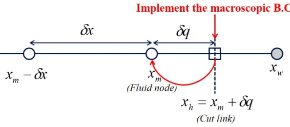
To apply the CBC to the MRT-LBM, the boundary conditions proposed by Ginzburg et al. In the present study, δq = 1/2 is assumed so that the boundary conditions have the second-order accuracy. In the LBM, the Dirichlet boundary condition for pressure is often used at the outlet points in which the incoming probability distribution function f¯i(xm, yk0, t) can be determined using the outgoing fi(xm, yk0, t).
For Dirichlet boundary conditions for LBM, the constant p(xh, yk0, t) =p0 and/or u(xh, yk0, t) = u0 are often applied and as such, may cause spurious flow behavior at the boundaries of open. . In the present study, instead, p(xh, yk0, t) and u(xh, yk0, t) are estimated at each time step by solving their evolution equations derived from the 2-D CBC, which will are explained below. section.
General formulation of the CBC
As such, L(x)i of the outgoing waves can be simply calculated by one-sided differences of Eq. The right choices of the relaxation coefficients are essential for the successful control of the wave reflection [33]. As such, the relaxation terms in Eq. 4.17 and 4.18 are supposed to give the boundary solutions to converge to desired target values in the steady limit of the flow, especially when the LODI assumption is valid at the boundaries.
To properly account for transverse and viscous terms in the boundary conditions, the original characteristic form of the NS equations must therefore be considered: For the evaluation of L(x)1 of the outgoing wave in Eq. 4.9 at the inlet, the derivatives are calculated using a second-order forward difference approach:
Result and Discussion
Vortex convection problem
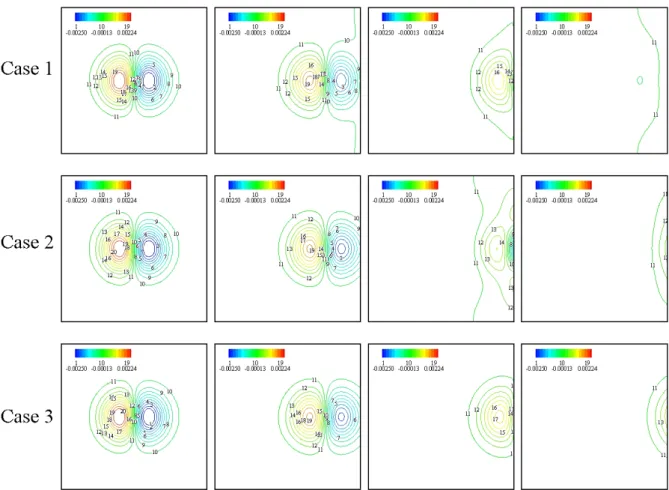
Note that the implementation of edge and corner treatments for 3-D CBC in [98] is so straightforward that it is not included here. From case 1 where the conventional CBC is used, it is easily seen that the vortex is distorted while passing through the outlet due to wave reflections created by the neglected transverse term. Although the recovery of the neglected transverse terms in case 2 improves the behavior by keeping the vortex shape longer, the flow distortion cannot be avoided at later times.
However, in case 3, where cross-member relaxation is also included, the vortex can pass through the outflow boundary without distorting the flow. These results are consistent with those found in conventional CFD simulations [34], confirming that 2-D CBC can effectively increase the accuracy and stability of the solution in LBM simulations.
Vortex shedding problem
Conclusion
36] ——, "Analysis of the Effects of Marangoni Stresses on the Microflow in an Evaporating Sedentary Drop," Langmuir, vol. Baigl, "Modulation of the Coffee Ring Effect in Particle/Surfactant Mixtures: The Importance of Particle-Interface Interactions," Langmuir, vol. Duan, "Elimination of the coffee ring effect by promoting particle adsorption and long-range interaction," Langmuir, vol.
Duan, "Three-dimensional Monte Carlo model of the coffee ring effect in evaporating colloidal droplets," Scientific Reports, vol. Luo, "Theory of the lattice Boltzmann method: Dispersion, dissipation, isotropy, Galilean invariance and stability," Phys.