Vol. 25, No. 1, 1–27, March 2011
The Performance of Industrial Policy:
Evidence from Korea
JAYMIN LEE
Department of Economics, Yonsei University, Seoul, Republic of Korea
(Received 21 June 2010; final version received 15 August 2010)
ABSTRACT This paper first shows that Korea implemented industrial policy properly, pro- moting infant industries rather than mature ones. The paper then shows that infant industries promoted by industrial policy have matured over time, as well as grown faster than mature industries not promoted by industrial policy. However, this happened as industrial policy was being lifted, rather than as it was being implemented. The paper also shows that, although industrial policy may pay off more easily than previously thought, Korean indus- trial policy fails to pay off because it distorted the price mechanism too severely and for too long. The analysis of the paper suggests that industrial policy in latecomer countries, when implemented to address market failure, should be much more moderate than what Korea implemented.
KEYWORDS: Industrial policy, infant industry, cost-benefit analysis, protection, subsidy JEL CLASSIFICATIONS: O25, F13, L52
1. Introduction
Industrial policy or ‘picking the winners’ by government has been discredited in developed countries. In developing countries, the experience of import sub- stituting industrialization in the 1950s and 1960s showed that industrial policy involved numerous government interventions whose overall impact on economic performance was disastrous. This led to the adoption of more liberal policies in developing countries, following the ‘Washington Consensus’. However, the per- formance of those developing countries that have adopted such policies, mostly
Correspondence Address: Jaymin Lee, Department of Economics, Yonsei University, 50 Yonseiro, Seodaemungu, Seoul 120–749, Republic of Korea. Email: [email protected]
1016-8737 Print/1743-517X Online/11/010001–27 © 2011 Korea International Economic Association DOI: 10.1080/10168737.2011.550122
in Latin America and Africa, has turned out equally disappointing. This has led many economists to examine the experiences of East Asian countries such as Japan, South Korea (henceforth Korea) and Taiwan. These countries not only experienced high economic growth but also implemented industrial policy at some stage of that high economic growth.
Most economists initially failed to pay attention to the fact that East Asian countries implemented industrial policy, attributing their high economic growth mainly to the working of free trade and, more broadly, unfettered market mech- anism. This view was challenged by some ‘revisionist’ writers who asserted that those economies had implemented industrial policy, and it was this that was responsible for their high growth performance (Johnson, 1982; Amsden, 1989;
Wade, 1990). The majority of economists have then come to recognize that East Asian countries did pursue industrial policy. However, these economists are appar- ently divided. Some insist that industrial policy has, if anything, only had a marginal effect (World Bank, 1993; Noland & Pack, 2003; Pack & Saggi, 2006).
Others think that industrial policy has had some beneficial effects (Rodrik, 1995, 1996, 2008; Stiglitz, 1996; Hausmann & Rodrik, 2003). As a result, the perfor- mance of industrial policy in the high performance East Asian economies is ‘by no means a settled debate, and the attempt to asses the impact of industrial policies remains a major area of research’ (Krugman & Obsfeld, 2006, p. 255).
That performance should be evaluated through empirical studies. There are three empirical questions to be addressed.
First, did East Asian countries implement industrial policy properly? This is seemingly an absurd question, but existing evidence casts doubts about the proper implementation of industrial policy in East Asia. For example, Beason and Weinstein (1996) show that in Japan, senile industries, rather than infant industries, captured the government and extracted more protection and subsi- dies. Japan was thus not so different from other countries where protection and subsidies were granted mainly for political reasons (Harrison & Rodríguez-Clare, 2009, pp. 34–35). It has also been questioned whether Korea implemented indus- trial policy properly. Korea followed a policy of promoting ‘heavy and chemical’
industries, but this policy proved extremely costly and was eventually judged to be premature and was abandoned (World Bank, 1993, p. 309; Krugman & Obsfeld, 2006, p. 255). Korean industrial policy could thus be regarded as only a half-baked one.
Second, have the industries promoted by industrial policy grown more rapidly and gained international competitiveness over time? This question is about whether the government has indeed managed to ‘pick the winners’, that is, infant industries that have grown and matured over time. It is important that the pro- moted industries grow faster because only by growing faster can they contribute to the high growth performance. However, of course, high growth without gaining international competitiveness is disastrous, as the experience of most developing countries has shown. Empirical studies have so far shown that industrial policy has not produced the maturation of infant industries in East Asian economies.
World Bank (1993, Chapter 6) and Pack (2000) show that protection and subsi- dies employed for the purpose of industrial policy have failed to have a positive effect on total factor productivity growth in East Asia. Lee (1996) reports the same results for Korea. In other words, empirical evidence for East Asia is little different
from the old evidence for other developing countries, which gave ‘an impression that there is not so much maturation of infants in very many developing countries’
(Bellet al., 1984, p. 103).
The third question is: has industrial policy paid off? This question is about the cost-benefit analysis of industrial policy. Is the benefit that accrues over time to promoted industries large enough to offset the cost of protection and subsidies that have helped them grow? This is the ultimate test of whether industrial policy contributes to the enhancement of welfare. Empirical study of this question has, so far, been out of the question. No method of cost-benefit analysis has been devised. There is only a suggestion that industrial policy is unlikely to pay off because of the effect of the discounting factor: the unit cost of promoted infant industries cannot fall faster than that of other industries at a rate higher than the social discount rate, which tends to be very high in developing countries (Krueger
& Tuncer, 1982, 1994).1
This paper will evaluate the performance of industrial policy in Korea. It will first show that Korea implemented proper industrial policy by promoting more dynamic infant industries in the name of the ‘heavy and chemical industry’ drive in the 1970s. The paper will then show that promoted infant industries grew more rapidly regardless of the halfway ‘abandonment’ of the policy, and that they have matured as well. It will then perform an ex post cost-benefit analysis and show that industrial policy in Korea nevertheless fails to pay off. In other words, the paper will show that Korea has managed to ‘pick the winners’, but at too high a cost.
The rest of the paper is organized as follows: section 2 describes the way Korean industrial policy was implemented and elaborates upon the analytical framework for the second and third questions raised above; section 3 shows that infant indus- tries promoted by industrial policy have matured, as well as grown faster than industries not promoted by industrial policy; section 4 carries out the cost-benefit analysis and shows that industrial policy fails to pay off; section 5 contains a discussion and concluding remarks.
2. Korean Industrial Policy and the Analysis of Its Performance 2.1 Korean Industrial Policy
Korea began its high economic growth with an export drive in the 1960s.
The exports mainly composed of unskilled-labor-intensive ‘light’ manufacturing goods. Then Korea began to build ‘heavy and chemical industries’ as a strat- egy to upgrade export structure. In the latter half of the 1960s and into the first years of the 1970s, there were various development activities in industries such as automobile, machinery, chemical, iron and steel, and shipbuilding. On January 30, 1973, the Korean government then formally launched the ‘heavy and chemi- cal industry’ drive, which was actually no more than a formal announcement of something that had already been happening. After the formal declaration of the
1There is one study that calculates the welfare effects of protecting a particular industry: the US tinplate industry in the late 19th century (Irwin, 2000). However, an empirical study about the industrial policy covering all of the manufacturing industries has not been conducted.
policy, across-the-board efforts were made from 1973 through 1978 employing various methods of protection, tax treatment, and credit rationing. The Korean government then began to ‘abandon’ the policy from April 1979, for the purpose of restoring macroeconomic stability. After a new government was installed in 1980, the policy was lifted in earnest, and sincere efforts were made for domestic liberalization and market opening. The move proceeded consistently thereafter, on Korea’s own initiative and with pressure from the US and other advanced countries. Liberalization and market opening accelerated under IMF surveillance after the East Asian crisis in 1997.
Some data are available to describe the incentive structure that the Korean government employed for industrial policy purposes during its implementation and subsequent lifting. The effective rate of protection (henceforth ERP) was calculated for 1970 by Kim and Hong (1982), and for 1975, 1978, 1980, 1983, 1985, 1988, 1990, 1993, and 1995 by Hong (1997). The classification of industries is completely consistent across these ten observations. The data for fiscal incentives are provided by Kwack (1985), who gives the data for effective corporate tax rate for promoted and non-promoted industries from 1970 to 1983. Since corporate tax exemptions and reductions were the major fiscal incentives (cash subsidies were rarely used), an effective corporate tax rate represents fiscal incentives (or disincentives) quite well. Meanwhile, no comprehensive data are available for the incentives provided by financial policy. In the 1960s and 1970s, Korea nationalized banks and implemented credit-rationing, setting official interest rates at a level far below the market-clearing ones. In addition, there were many ‘policy loans’
on which the government set interest rates further below the market clearing ones.
However, the exact amount of the margin of the subsidy provided through credit rationing has not been calculated. The closest approximation of that margin for which data are available is the difference in the average cost of borrowing between promoted and non-promoted industries. It should reflect, if not totally, the effect of credit rationing for industrial policy.
Table 1 gives the effective rate of protection, the effective corporate tax rate, and the average cost of borrowing for promoted and non-promoted industries.
Their differences are also presented, since what matters as an incentive in resource allocation is the difference rather than the absolute level itself.
The manufacturing sector is classified into two groups of promoted and non- promoted industries rather than classified as individual industries. In the 1970s, the Korean government promoted the entire group of ‘heavy and chemical indus- tries’ rather than just one or two industries. Uncertainty about the future is inherent in all industrial development, with some industries doing better than expected and others worse. What matters, therefore, in an industrial policy, such as Korea’s in the 1970s, is whether the overall policy efforts will result in a performance of promoted industries above the level achieved in non-promoted industries (Stern et al., 1995, p. 11). Promoted industries consist of chemicals, metals, machinery (including electronic machinery), and transportation equip- ment. Non-promoted industries include the rest of manufacturing industries:
food, textile, garments, footwear, and wood products, among others.
One problem here is the possibility that the contents of industries may change over time. This is particularly true for promoted industries, which contain tech- nologically more dynamic industries. The ‘heavy and chemical industries’ in the
ThePerformanceofIndustrialPolicy5
Unit: percent Effective rate of protection Effective corporate tax rate Average cost of borrowing Year Promoted Non-promoted Difference Promoted Non-promoted Difference Promoted Non-promoted Difference
1970 25.5 8.7 16.8 39.2 39.4 −0.2 17.7 15.5 2.2
1971 34.9 34.7 0.2 12.9 14.4 −1.5
1972 27.7 29.8 −2.1 10.5 13.3 −2.8
1973 33.5 38.6 −5.1 8.7 10.9 −2.3
1974 29.9 37.7 −7.8 10.4 10.6 −0.2
1975 6.8 −15.1 21.9 15.9 52.1 −36.2 10.2 12.2 −1.9
1976 18.0 51.0 −33.0 10.1 13.7 −3.6
1977 17.5 49.5 −32.0 11.5 14.3 −2.8
1978 37.4 −5.7 43.1 16.9 48.4 −31.5 10.1 15.9 −5.8
1979 18.3 48.5 −30.2 12.5 16.6 −4.1
1980 44.2 10.7 33.5 18.3 48.8 −30.5 17.6 20.1 −2.5
1981 20.6 51.1 −30.5 17.5 19.6 −2.2
1982 47.1 48.2 −1.1 15.3 16.9 −1.6
1983 26.2 8.7 17.5 40.4 42.2 −1.8 12.9 14.6 −1.7
1984 14.4 14.5 −0.1
1985 15.2 −2.5 17.7 12.7 14.8 −2.0
1986 12.0 13.5 −1.6
1987 12.1 13.4 −1.3
1988 9.9 −13.5 23.4 12.7 13.6 −0.9
1989 13.5 13.8 −0.2
1990 12.9 −5.8 18.7 12.5 13.1 −0.5
1991 12.7 13.5 −0.8
1992 11.9 13.2 −1.4
1993 6.6 −0.9 7.5 10.9 12.0 −1.2
1994 11.1 12.3 −1.2
1995 3.9 −1.3 5.2 11.3 12.8 −1.5
1996 10.9 12.2 −1.3
Data: 1) Effective rate of protection calculated from Kim and Hong (1982) and Hong (1997).
2) Effective corporate tax rate from Kwack (1985).
3) Average cost of borrowing from the Bank of Korea,Financial Statements Analysis.
early 1970s were composed of smokestack industries or lower-end activities of higher technology industries, but their contents changed over time. For example, the Korean electronics industry consisted mainly of product assembly, such as that of TV sets and transistor radios in the 1970s; however, Korea developed semicon- ductor memory chips in the 1980s and LCDs (liquid crystal displays) and FPDs (flat panel displays) in the 1990s. The Korean automobile industry developed a front-wheel drive car in the 1980s. However, the development of these new prod- ucts was mainly based on the accumulated technological capabilities within the electronics industry and the automobile industry. If some cross-industry exter- nality was a factor in the development of those products, it came most likely from other promoted industries: in Korea, interactions among individual industries within each of the promoted and non-promoted industries far exceed the inter- actions between any individual promoted industry and individual non-promoted industry (Pack, 2000).
Classifying the manufacturing sector into two groups is also consistent with the aim of Korean industrial policy. The aim of Korean industrial policy was not acquiring comparative advantage in smokestack industries or lower-end activities of higher technology industries. It was eventually acquiring comparative advan- tage in the very high technology products in the high technology industries. In other words, the Korean government wanted to ‘catch up’ with advanced countries through industrial policy.
Table 1 shows that promoted industries received higher ERP than non- promoted ones, as of 1970. Until 1978, the gap in the ERP widened to 43.1 percentage points, reflecting the all-out implementation of industrial policy. The gap was then narrowed as the industrial policy was lifted from 1979 onwards. It continued to fall, although with some fluctuations, as market opening proceeded.
The difference in effective corporate tax rate shows a more drastic rise and fall. It began to rise in 1973 to reach more than 30 percentage points by 1975 and stayed there until 1981, before falling abruptly to less than 2 percentage points in 1982 and 1983. The difference in the average cost of borrowing shows a less drastic but similar trend. It rose from 1971 and stayed at a relatively high level from 1976 to 1979 and then fell more gradually than the difference in effective corporate tax rate. Of course, we cannot be sure that this trend of average cost of borrowing solely reflects the effect of credit rationing for industrial policy. However, we have the estimates of the weight of policy loans in domestic credit, which are presented in Appendix Table 1A. The broad picture that emerges out of those estimates is that the weight of policy loans rose in the 1970s and fell from the 1980s.2
2This may be complicated by the existence of a policy loan that was important but not related to industrial policy, i.e. loans for exports. Loans for exports remained neutral across the promoted and non-promoted industries, but they may have affected the difference in the average cost of borrowing if its composition differed between the promoted and non-promoted industries. The composition of the loans for exports should have depended on the composition of exports themselves. The share of promoted industries in total manufacturing exports was lower than 50% from 1970 to 1978 (shown later). The lower average cost of borrowing for promoted industries, in spite of a lower proportion of loans for exports, means that the credit rationing for loans other than exports favored the promoted industries. It is less clear that credit rationing for industrial policy accounted for the lower average cost of borrowing for promoted industries after 1978 because of the higher export
In summary, the figures in Table 1 fit the above description of the process of implementation and ‘abandonment’ of industrial policy: the policy was initiated from around 1970; all-out efforts were made from 1973 to 1978; and it was lifted subsequently.
2.2 Analytical Framework
To evaluate the performance of Korean industrial policy, we have first to analyze the trend of the growth rate of promoted industries as compared with that of non-promoted industries, not only during the period when industrial policy was implemented but also during the period when it was lifted. This will be relatively simple, given the data on the growth rates of industries.
We then have to analyze whether promoted industries have acquired inter- national competitiveness over time. The essence of this analysis is illustrated in Figure 1. UCP(t)in Panel (A) of Figure 1 represents unit cost curve of pro- moted industries. UCP(t)is normalized by the unit cost of the same industries in the world market, denoted asUC∗P(t). Since industrial policy promotes infant industries,UCP(t)is larger than one (1.0) at the initial point of time, when the industrial policy is undertaken — denoted as ‘0’ in Figure 1. The incentive mea- sures described in Table 1 allow the promoted industries to have such a high unit cost.
For the promoted infant industries to mature,UCP(t) should fall below one over time before production expires in the remote future, which is denoted as F.
However, in the general equilibrium context, UCP(t)should be larger than the unit cost of non-promoted industries initially but should become smaller than the unit cost of non-promoted industries over time. This relationship is presented in Panel (B) of Figure 1.UCP(t)is replicated as the dotted line. The unit cost of non-promoted industries is denoted asUCN(t), which is also normalized by the unit cost of the same industries in the world market, denoted asUC∗N(t). Testing the maturation of promoted infant industries is thus equivalent to finding the point of time ‘M’.
Testing whether industrial policy pays off is more complicated. If there were no discounting problems, the net benefit of the promoted industries is equivalent to the size of the area CDE minus that of the area ABC in Panel (A) of Figure 1.
Of course, the former should be discounted in relation to the latter because it is realized later. However, the effect of the social discount rate could be offset by that of output growth. Future cost savings may have to be discounted in order to be compared with the present loss caused by higher unit cost, but the former will be larger because of output growth. If the growth rate of output is sufficiently larger than the social discount rate after the promoted infant industries mature, cumulative benefits may outweigh cumulative costs. Owing to the effect of output growth, the possibility that net benefit of promoted industries may be positive is higher than previously thought. Of course, in a general equilibrium context, the net benefit of the promoted industries should be compared with the net benefit of
share of promoted industries. Anyway, all credit rationing was phased out from the 1980s, and this should be responsible for the shrinking difference in the average cost of borrowing.
(A) Promoted industries
(B) Non-promoted industries unit cost
1.0
UCp (t) UCp
* (t)
0 F
E D B
C A
unit cost
1.0
UCp (t) UCN*
(t)
0 F
K I J
G
UCN (t)
M H
Figure 1.The trend of unit cost.
the non-promoted industries. The net benefit of non-promoted industries can be calculated in a similar way, by comparing the areas GHI and IJK in Panel (B) of Figure 1, after adjusting for the discount and growth rates. Industrial policy will pay off if the net benefit of the promoted industries outweighs the net benefit of non-promoted industries.
This paper will show that Korean industrial policy fails to pay off in spite of the fact that the possibility for industrial policy to pay off is higher than previously thought. It will do so by conducting an ex post cost-benefit analysis, taking the trends of unit cost, output growth, and the social discount rate into account.
The initial point of time, denoted as ‘0’ in Figure 1, is set to the date when the Korean government began to implement industrial policy. The date ‘0’ is not set at the time when production began: tracing the production of promoted and non-promoted industries to their very beginning is not only impossible, but also irrelevant, since our major concern is the evaluation of the performance of industrial policy. Considering the process of the unfolding of the industrial policy described above, the date ‘0’ is set at two alternative points of time. First, ‘0’ is set at the beginning of 1970 because it is a point of time between the late 1960s
and early 1970s, and because the data for the unit cost are available from 1970 (explained below). Second, ‘0’ is set at the beginning of 1973, when the ‘heavy and chemical industry’ drive was formally launched. The trend ofUCP(t)andUCN(t) from 1970 or 1973 on will indicate whether promoted infant industries mature.
To see whether the policy paid off, we carry out cost-benefit analysis from the beginning of 1970 or 1973, treating the cost and benefit incurred earlier as the sunk cost or benefit. Meanwhile, it is out of the question to trace the trajectory of the unit cost and the output into the remote future when production expires — denoted as F in Figure 1. However, we can calculate the values of the unit cost and output to the extent that data allow and make some inferences from them.
There are a few problems to be clarified in implementing the cost-benefit analysis referring to Figure 1, after modifying it for discounting and growth.
First, the cost-benefit analysis does not capture the allocative inefficiency caused by the distortion of the price mechanism in each year. However, being incurred during the period of implementing industrial policy, it adds to the cost of industrial policy. If the calculated net benefit is negative, adding the cost of allocative inefficiency will reinforce the conclusion that industrial policy fails to pay off.
Second, the cost-benefit analysis does not capture all the government interven- tion in the financial sector. The amount of subsidies provided by credit rationing is considered in the calculation of unit cost and is taken into account in the cost- benefit analysis. However, there are other (indirect and unintended) costs. As a result of nationalization, banks came to lose independent entity as business, and thus were unable to monitor and discipline firms in the 1970s. Although banks were formally privatized in the 1980s, government influence persisted. Under this situation, firms were not much interested in raising profitability while they depended heavily on borrowing for investment. This led to sporadic financial crises, which inflicted a large cost on the economy. We will avoid this problem by showing that industrial policy fails to pay off even if that cost is excluded.
Third, if net benefit is large enough, private firms will enter the promoted industries on their own calculation of cost and revenue. Industrial policy is unnecessary. It is legitimate only when there are market imperfections, such as knowledge spillovers, dynamic scale economies, coordination failures, and infor- mation asymmetries, which are typical grounds for the infant industry argument (Hausmann & Rodrik, 2003; Melitz, 2005; Sauré, 2007; Harrison & Rodríquez- Clare, 2009). However, this is not a problem either, since the purpose of this paper is to show that Korea’s industrial policy fails to pay off. It would be meaningful to ask whether the industrial policy addressed market failure correctly only when industrial policy pays off. If it fails to pay off, the policy is illegitimate whether it addressed market failure correctly or not. Of course, this will matter when we dis- cuss the implications of the analysis to industrial policy for latecomer countries, which is mentioned in section 5.
3. The Growth and Maturation of Infant Industries
This section investigates the performance of industrial policy as manifested by the growth and maturation of promoted infant industries. For that purpose, we
have to examine the growth pattern and the trend of unit costs for promoted and non-promoted industries.
The data for the growth of industries are available from the Bank of Korea.
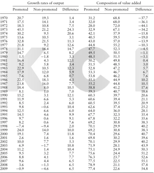
Table 2 presents the growth rates of output (in constant prices) and the composi- tion of value added (in current prices) for promoted and non-promoted industries.
The growth of promoted industries accelerated both in absolute terms and in
Table 2.Growth rates of output and the composition of value added
Unit: percent Growth rates of output Composition of value added Promoted Non-promoted Difference Promoted Non-promoted Difference 1970 20.7 19.3 1.4 31.2 68.8 −37.7 1971 17.5 14.1 3.4 32.0 68.0 −36.1 1972 18.3 10.8 7.5 28.0 72.0 −44.1 1973 45.5 21.2 24.3 32.9 67.1 −34.2 1974 30.2 9.5 20.6 42.1 57.9 −15.8 1975 13.6 10.5 3.1 40.5 59.5 −19.0 1976 32.8 21.5 11.3 43.0 57.0 −13.9 1977 21.8 9.2 12.6 44.8 55.2 −10.3
1978 31.1 16.4 14.7 47.7 52.3 −4.5
1979 14.7 6.5 8.2 49.5 50.5 −1.1
1980 1.5 −1.8 3.3 48.5 51.5 −3.1
1981 16.4 4.3 12.1 50.2 49.8 0.4
1982 9.2 5.8 3.4 51.5 48.5 3.0
1983 22.9 10.5 12.3 52.8 47.2 5.7
1984 17.9 12.0 5.9 53.3 46.7 6.7
1985 7.6 6.8 0.7 53.8 46.2 7.6
1986 22.5 18.3 4.3 55.1 44.9 10.2
1987 23.8 16.0 7.7 55.2 44.8 10.5
1988 18.4 8.0 10.5 58.8 41.2 17.6
1989 8.1 1.0 7.0 59.3 40.7 18.6
1990 15.2 3.1 12.1 60.3 39.7 20.6
1991 11.9 6.6 5.3 60.6 39.4 21.1
1992 8.5 2.4 6.0 60.5 39.5 20.9
1993 9.8 −0.6 10.4 62.6 37.4 25.2
1994 12.5 6.6 6.0 64.0 36.0 28.1
1995 14.5 4.6 9.9 67.7 32.3 35.4
1996 9.7 0.6 9.1 67.8 32.2 35.6
1997 8.2 0.6 7.6 69.2 30.8 38.3
1998 −7.4 −9.4 2.0 70.1 29.9 40.2
1999 24.0 14.0 10.0 69.2 30.8 38.3
2000 19.1 7.4 11.8 70.4 29.6 40.7
2001 2.6 1.6 1.6 69.8 30.2 39.6
2002 10.0 7.7 5.3 70.1 29.9 40.2
2003 6.9 −1.7 10.8 71.9 28.1 43.9
2004 11.2 1.4 10.4 75.1 24.9 50.3
2005 9.5 3.2 7.7 75.6 24.4 51.2
2006 8.8 4.1 7.7 76.3 23.7 52.6
2007 9.6 4.4 6.5 77.5 22.5 55.1
2008 3.6 −1.3 6.5 78.9 21.1 57.8
2009 −0.9 −4.6 6.5 77.4 22.6 54.8
Notes: 1) Growth rates of output at constant process with 1975, 1985, 1995 and 2005 for 1970s, 1980s, 1990s and 2000s respectively. Composition of value added in current prices.
Data: The Bank of Korea.
relation to non-promoted industries from 1970 to 1978. Then, from 1979, the growth of promoted industries decelerated. This acceleration and deceleration of the growth of promoted industries is apparently the result of the implementation of the industrial policy and its subsequent lifting, as described above. It is not surprising that the growth of promoted industries accelerated as industrial policy was implemented from 1970 to 1978. However, it is notable that the deceleration of the growth of promoted industries with the lifting of industrial policy did not mean a lower growth rate of promoted industries in relation to non-promoted ones. The ‘abandonment’ of the industrial policy did not mean the abandonment of the promoted industries themselves. Because of the higher growth of promoted industries, their share of value added also rose drastically, from about 31% in 1970 to about 79% in 2008.
To measure the trend of the unit cost, previous studies of industrial policy (and related topics) have examined the trend of total factor productivity growth (Krueger & Tuncer, 1982; Bellet al., 1984; Harrison, 1994; Beason & Weinstein, 1996; Lee, 1996; Pack, 2000). However, total factor productivity growth does not account for all of the change in unit cost. The change in unit cost depends on the change in factor use and the change in the terms of trade, as well as total factor productivity growth. The change in the terms of trade is, in turn, affected by the change in factor use and total factor productivity growth of overseas producers competing with domestic producers. This has been confirmed by Nishimitsu and Page (1986), who show, using data from Thai manufacturing industries, that domestic total factor productivity growth accounts for an important part, but by no means all, of the change in unit cost.
A more accurate and straightforward way is to calculate the trend of the unit cost itself as illustrated in Figure 1. A useful measure with which to begin, in this regard, is the extent to which the domestic price is higher than the world market price, that is, the nominal rate of protection (henceforth NRP):
NRPi(t)=Pdi(t)/P∗i(t)−1 (1) where
NRPi(t)=nominal rate of protection at timet, Pdi(t)=domestic market price at timet, P∗i(t)=world market price at timet, and
i =P,N, withPandNeach denoting promoted and non-promoted industries, respectively.
However, in small open economies, which import considerable amounts of intermediate inputs, the ERP, which takes the protection on inputs into consideration, is more appropriate than the NRP:
ERPi(t)=
⎡
⎣NRPi(t)−
j
NRP(t)aji
⎤
⎦
⎛
⎝1−
j
aji
⎞
⎠
=(DVAi(t)−WVAi(t))/WVAi(t)−1 (2)
where
ERPi(t)=effective rate of protection at timet,
DVAi(t)=value added in domestic market prices at timet, WVAi(t)=value added in world market prices at timet, aji(t)=input coefficient at timet, and
i,j =P,N.
To use the ERP as a measure of unit cost, the NRP used to calculate it should be measured by a comparison of domestic and world market prices rather than by the magnitude of the tariff rate. Fortunately, the ERP figures presented in Table 1 have been calculated using the NRP based on a comparison of domestic and world market prices.3
However, these figures of the ERP have two limitations as a proxy of unit cost.
First, the ERP, as well as the NRP, are affected by currency overvaluation or undervaluation. To cope with this problem, we revise the ERP figures by referring to the ERP of the whole manufacturing sector.
ERPRi(t)=(ERPi(t)+1)/(ERPA(t)+1)−1
= [(DVAi(t)−WVAi(t))/WVAi(t)]/[(DVAA(t)
−WVAA(t))/WVAA(t)] −1 (3)
where
ERPRi(t)=revised ERP at timet,
ERPA(t)=ERP of the whole manufacturing sector at timet,
DVAA(t)=value added of the whole manufacturing sector in domestic market prices at timet,
WVAA(t)=value added of the whole manufacturing sector in world market prices at timet,
i,j =P,N.
Utilizing the ratio(ERPi(t)+1)/(ERPA(t)+1)eliminates the problem of cur- rency overvaluation or undervaluation.ERPRi(t)represents the relative departure of value added in domestic market prices from value added in world market prices between the promoted or non-promoted industries and the whole manufactur- ing sector.ERPRi(t)thus measures the relative efficiency in resource allocation between promoted and non-promoted industries and the whole manufacturing sector.4
3To represent the unit cost, the ERP should be calculated for total sales rather than domestic sales only. Kim and Hong (1982) provide the ERP data for both domestic and total sales, but Hong (1997) only for domestic sales. We thus calculate the ERP for total sales from Hong’s (1997) data as the weighted average between domestic sales and exports, using domestic sales in world market prices (that is, (domestic sales)/(1+NRPi(t))) and exports as weights. All ERP figures are calculated by the Corden method. Using the Balassa method does not alter the conclusion of the paper.
4Equation (3) reduces the comparison of unit cost between domestic producers and foreign pro- ducers into a comparison of the unit cost between promoted (or non-promoted) industries and the whole manufacturing sector. They are actually equivalent to each other because what matters in both of them is efficiency in the allocation of domestic resources (Bruno, 1972).
The second limitation of the ERP as a proxy of unit cost is that the ERP is calculated by comparing prices so that it overestimates unit cost by the net profit margin. This is especially problematic considering that, over time, the revised ERP of both promoted and non-promoted industries will converge towards zero as market opening proceeds, and the difference in unit cost will mainly be accounted for by the difference in net profitability. The benefit of industrial policy after the promoted infant industries mature will, therefore, take the form mainly of a difference in net profitability. Net profitability is calculated as follows:
πi(t)= [GPi(t)−ck(t)TKi(t)]/DVAi(t)
=GPi(t)/DVAi(t)−ck(t)TKi(t)/DVAi(t) (4) where
πi(t)=net profitability (the ratio of net profit to domestic value added) at timet, GPi(t)=gross profit (profit before tax + interest paid) at timet,
ck(t)=cost of capital at timet, TKi(t)=total capital at timet, and i =P,N.
Net profitability is defined as net profit divided by value added in domestic market prices. Net profit is measured as gross profit subtracted by the total cost of capital. Gross profit is calculated as profit before tax plus interest paid, and the total cost of capital is calculated by the cost of capital multiplied by total capital.
Net profitability calculated by equation (4) is not the same as the net prof- itability actually enjoyed by firms. It is based on the profit before, rather than after, tax, and the cost of capital is the (social opportunity) cost of capital for the whole economy, rather than the cost of capital actually incurred by firms. This is done to eliminate the effect of subsidies. If the actual profitability of promoted industries is higher due to subsidies (tax exemptions and deductions, and lower interest rates due to credit rationing), it will reduce the actual unit cost for the promoted industries, but this does not mean that their opportunity cost in terms of resource allocation, which is our major concern, is reduced. Since corporate tax exemptions and reductions were the major fiscal incentives, using profit before, rather than after, tax will largely eliminate the effect of fiscal subsidies. Using the cost of capital for the whole economy rather than the cost of the capital actually incurred by firms will account for the effect of financial subsidies.
The data for GPi(t)/DVAi(t) and TKi(t)/DVAi(t) are available for all years from the Bank of Korea’sFinancial Statement Analysis. The data situation for the cost of capitalck(t)is much worse. While it was calculated for some years in the 1960s and 1970s (Hong, 1979, Chapter 7), data covering all the years are not available. The figure that is closest to the cost of capital for which data are available for all the years is the ‘average cost of borrowing in the whole manufacturing sector’, which is provided in theFinancial Statement Analysis. Of course, this is a poor approximation. The average cost of borrowing for the ‘whole manufacturing sector’ would be different from the average cost of capital for the ‘whole economy.’
More importantly, the average cost of borrowing should underestimate the cost
of equity capital by the margin of the premium for business uncertainty. However, given the data situation, it seems the closest proxy of the cost of capital.5
The unit cost is calculated as follows:
UCi(t)= [1+ERPRi(t)][1−πi(t)] (5) Regarding the years for which ERP data are missing, approximate figures of UCi(t) can be calculated by filling in the missing ERP figures through interpolation.
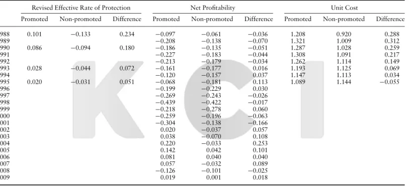
Table 3 presents the revised ERP, net profitability, and unit cost. The difference of each variable between promoted industries and non-promoted industries is also presented, considering that what matters in the general equilibrium context is the difference rather than absolute level.
The trend of the difference in the revised ERP is similar to that of the ERP itself.
It rose to its maximum at 0.394 in 1978 and then began to fall until it reached a point as low as 0.051 in 1995.
Promoted industries had lower net profitability than non-promoted industries from 1970 to 1978, except in 1974, often by a large margin. The net profitability of promoted industries was lower than that of non-promoted industries by a large margin in the 1970s and peaked in 1980, probably showing that firms entered pro- moted industries by being attracted by subsidies rather than profitability (before subsides). The margin then narrowed from 1981, with the phasing out of the sub- sidies through the 1980s. It became positive from 1993 to 1996, but again turned negative for a few years from 1997, the year when the East Asian crisis occurred, apparently because the net profitability of ‘heavy and chemical industries’ was more sensitive to the crisis. The margin became consistently positive from 2002 to 2007, after the recovery from the crisis in 1997. It has become negative again in 2008 because of the global crisis.
The trend of unit costUCi(t)reflects the trend of the revised ERP and net prof- itability. From 1970 to 1973,UCP(t)is larger thanUCN(t). This confirms that the
‘heavy and chemical industries’ promoted by the Korean government in the 1970s were indeed infant industries, while ‘light industries’ not promoted by the gov- ernment were mature industries.6The difference in unit cost UCP(t)−UCN(t) increased in the 1970s, peaking in 1980. It then began to shrink from 1981 on, and eventually became negative in 1995, implying that promoted infant indus- tries matured by 1995. However, it is not easy to conclude that they matured in 1995. The difference in unit cost became negative in 1995 because of the unusually large difference in net profitability, reflecting the high profitability of the promoted industries, probably owing to an unusual boom in the semiconductor industry
5One may wonder how the average cost of borrowing could be used as a proxy of the cost of capital for the 1970s when there was a large amount of subsidies because of credit rationing. However, credit rationing to some particular firms or industries meant that firms or industries unable to access official credit had to resort to borrowing from the curb market, which carried much higher interest rates than the market-clearing one. Therefore, for the economy as a whole, it is questionable whether credit rationing lowered the average cost of borrowing.
6Owing to short-term fluctuations in net profitability,UCN(t)is larger than one in 1970 and 1971.
However, the average ofUCN(t)from 1970 to 1973 is 0.958, and the average ofUCN(t)from 1970 to 1979 is 0.930. This suggests that the non-promoted industries were mature industries in the 1970s.
ThePerformanceofIndustrialPolicy15
Revised Effective Rate of Protection Net Profitability Unit Cost
Promoted Non-promoted Difference Promoted Non-promoted Difference Promoted Non-promoted Difference
1970 0.088 −0.057 0.146 −0.162 −0.143 −0.019 1.265 1.078 0.187
1971 −0.302 −0.150 −0.152 1.422 1.072 0.350
1972 −0.229 −0.039 −0.190 1.347 0.958 0.390
1973 0.069 0.205 −0.136 1.025 0.723 0.301
1974 0.076 −0.041 0.117 1.021 0.934 0.087
1975 0.110 −0.117 0.228 −0.084 −0.063 −0.021 1.203 0.938 0.265
1976 −0.106 −0.014 −0.092 1.286 0.887 0.399
1977 −0.128 −0.052 −0.076 1.309 0.938 0.372
1978 0.255 −0.139 0.394 −0.132 0.037 −0.169 1.420 0.829 0.591
1979 −0.189 −0.052 −0.137 1.468 0.945 0.522
1980 0.216 −0.067 0.282 −0.523 −0.227 −0.296 1.852 1.145 0.706
1981 −0.409 −0.234 −0.175 1.659 1.157 0.502
1982 −0.326 −0.244 −0.082 1.491 1.173 0.318
1983 0.097 −0.055 0.152 −0.186 −0.117 −0.069 1.302 1.056 0.246
1984 −0.191 −0.165 −0.026 1.288 1.076 0.212
1985 0.064 −0.100 0.163 −0.180 −0.123 −0.057 1.255 1.011 0.244
1986 −0.108 −0.027 −0.081 1.192 0.914 0.278
1987 −0.132 −0.015 −0.117 1.237 0.888 0.349
(Continued)
J.Lee
Table 3.Contiuned
Revised Effective Rate of Protection Net Profitability Unit Cost
Promoted Non-promoted Difference Promoted Non-promoted Difference Promoted Non-promoted Difference
1988 0.101 −0.133 0.234 −0.097 −0.061 −0.036 1.208 0.920 0.288
1989 −0.208 −0.138 −0.070 1.321 1.009 0.312
1990 0.086 −0.094 0.180 −0.186 −0.135 −0.051 1.287 1.028 0.259
1991 −0.227 −0.183 −0.044 1.308 1.091 0.217
1992 −0.213 −0.179 −0.034 1.262 1.114 0.149
1993 0.028 −0.044 0.072 −0.161 −0.177 0.016 1.193 1.125 0.069
1994 −0.120 −0.157 0.037 1.147 1.113 0.034
1995 0.020 −0.031 0.051 −0.068 −0.181 0.113 1.089 1.144 −0.055
1996 −0.199 −0.229 0.030
1997 −0.269 −0.243 −0.026
1998 −0.439 −0.422 −0.017
1999 −0.218 −0.278 0.060
2000 −0.259 −0.196 −0.063
2001 −0.304 −0.138 −0.166
2002 0.020 −0.037 0.057
2003 0.038 −0.070 0.108
2004 0.220 −0.033 0.253
2005 0.142 0.042 0.101
2006 0.081 0.040 0.040
2007 0.057 −0.032 0.089
2008 −0.126 −0.101 −0.025
2009 0.019 0.001 0.018
Notes: 1) Unit cost figures for which the data for effective rate of protection is unavailable are calculated by interpolation.
Data: 1) Net profitablity calculated from the Bank of Korea,Financial Statement Analysis.
that year. The difference in net profitability became much smaller in 1996 and neg- ative in 1997. Unfortunately, no data of the revised ERP are available after 1995.
However, some inference about the trend of the difference in unit cost after 1995 can be made from the data of the revised ERP and net profitability. After 1995, the difference in the revised ERP should fall from its level of 0.051 in 1995 because of market opening. Thus, if the difference in net profitability becomes larger than 0.051 after 1995, the difference in unit cost will surely become negative. This is the case from 2002 to 2007, with the exception of 2006. The difference in net profitabil- ity in 2006 is 0.040, which does not fall far short of 0.051. The difference became
−0.025 in 2008, apparently because of the global crisis. If we recognize that 2008 is probably abnormal, we could say that Korean infant industries promoted by industrial policy are most likely to have matured sometime from 1995 to 2007.
This empirical result confirms intuitive observations. Korea has undergone a rapid structural transformation of revealed comparative advantages. Korea exported mainly garments, textiles, veneers, and toys in the 1970s, but has come to export mainly automobiles, steel, ships, chemical products, and electronic goods over the years. The share of promoted industries in total manufacturing exports was 37.5% in 1970, 38.8% in 1975, 40.7% in 1978, 52.0% in 1980, 61.2%
in 1985, 59.5% in 1990, and 83.1% in 2000. Of course, the changing structure of revealed comparative advantage means changing international competitive- ness only when subsidies are being lifted. Thus, the rising subsidies, rather than improved international competitiveness, may have been responsible for the ris- ing export share of the promoted industries in the 1970s, but falling subsidies should not be responsible for their rising share from the 1980s. The change of revealed comparative advantage from the 1980s should be the result of improved international competitiveness of promoted industries.
To summarize the results presented in Tables 2 and 3, infant industries pro- moted by industrial policy have grown and matured. Korea has indeed succeeded in ‘picking the winners’.
4. Cost-Benefit Analysis
To see whether industrial policy pays off, we carry out ex post cost-benefit analysis by taking into account the growth rate of output and social discount rate, as well as the trend of the unit cost. The cumulative net benefit of promoted and non-promoted industries, denoted asCNBi, can be calculated as follows:
CNBi = F
0
NBi(t)dt (6)
NBi(t)=(1−UCi(t))e
t
0gi(s)dse−rt (7)
where
NBi(t)=net benefit at timet,
gi(s)=growth rate of real output at times, r =social discount rate,
i =P,N.
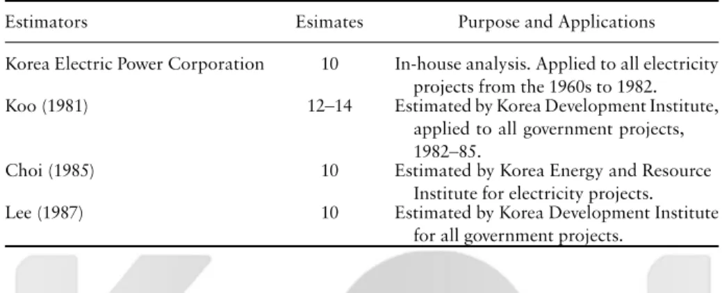
For industrial policy to pay off,CNBPshould be larger thanCNBN. Since the figures for unit cost and the growth rate of output are already available, net benefit NBi(t)can be calculated if the figures for social discount rate are available. The Korean government never declared the social discount rate applied to industrial policy. However, some estimations of the social discount rate were made for other purposes from the 1960s to the 1980s, as shown in Table 4.
Table 4.Social discount rates
Unit: percent
Estimators Esimates Purpose and Applications
Korea Electric Power Corporation 10 In-house analysis. Applied to all electricity projects from the 1960s to 1982.
Koo (1981) 12–14 Estimated by Korea Development Institute,
applied to all government projects, 1982–85.
Choi (1985) 10 Estimated by Korea Energy and Resource
Institute for electricity projects.
Lee (1987) 10 Estimated by Korea Development Institute
for all government projects.
Two out of the four estimates presented in Table 4 were associated with the Korea Electric Power Corporation projects, the state enterprise in charge of build- ing electricity projects, while the other two were associated with all government projects. There is hardly any reason to believe that the social discount rate applied to industrial policy should differ from these rates. The figures in Table 4 thus sug- gest that the social discount rate is 10% or higher. We set the social discount rate at 10%, considering that only one estimate (Koo, 1981) is higher than 10%.
Table 5 presents each of the two values of net benefitNBi(t) calculated by setting ‘0’ at the beginning of 1970 and 1973. The cumulative sum ofNBi(t)up to a certain year is also presented.
We first focus on the case where ‘0’ is set at the beginning of 1970. In this case, the net benefit of promoted industriesNBP(t)is consistently negative from 1970 to 1995, and the sum ofNBP(t)from 1970 to 1995 is−27.487. Meanwhile, the sum of the net benefit of non-promoted industries NBN(t) from 1970 to 1995 is−0.001. The cost of industrial policy incurred from 1970 to 1995 is thus 27.487−0.001=27.486. Unfortunately, it is impossible to calculateNBP(t)and NBN(t)beyond 1995 because of a lack of ERP data. It is possible, however, to have some idea about their magnitude by making use of the information about the trend of output growth in Table 2 and net profitability in Table 3. Examination of the trend of output growth and net profitability suggests that the cost of industrial policy incurred from 1970 to 1995 is unlikely to be recovered.
An illustration based on some assumptions about the trend of unit cost and the growth rate of output beyond 1995 may elucidate this idea. The trick here is to make assumptions favorable to industrial policy and then show that the cumulative net benefit of promoted industries is unlikely to be larger than that of non-promoted industries even under those assumptions.