53 The lateral position response of the platoon family of MRVs: (a) Steering angle family with step input, (b) Lateral position family with step input ··· 102 Fig. 54 The multi-destination lateral responses of the platoon family of MRVs:. a) the responses to the lateral position. (b) Input signal for lateral control.··· 103 Fig.

Introduction
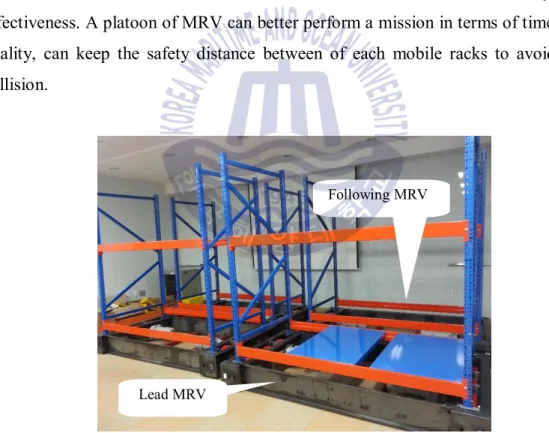
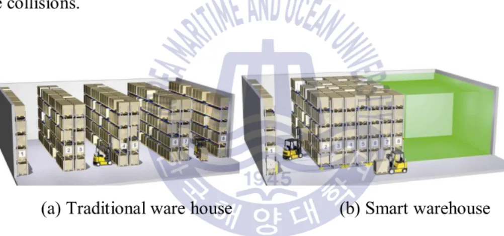
Mobile rack vehicle
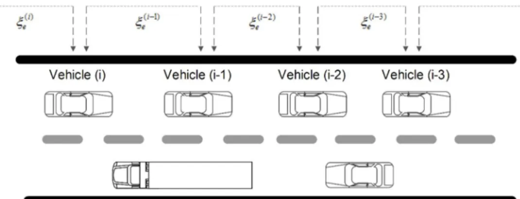
In the fully automated process of a mobile rack vehicle system, the user sets the desired position and velocity of the main vehicle. A distance sensor and the encoder attached to the front of the rack and the axle of the wheel are used to measure the preceding mobile rack distance and velocity, respectively.
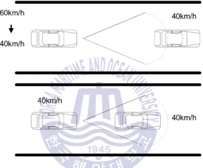
Leader and following vehicle
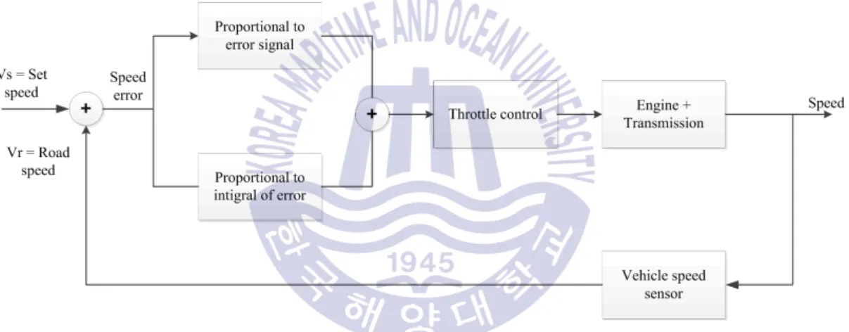
- Cruise control
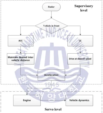
- Adaptive cruise control
- String stability of longitudinal vehicle platoon
- String stability of lateral vehicle platoon
Finally, the changes in the position of the throttle lead to the change in the speed of the car and achieve the desired speed. The lateral deviation of the preceding vehicle is transferred to the vehicle immediately following it, as shown in fig.
Problem definition
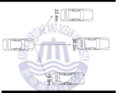
Radar signals are very good at detecting objects that strongly reflect electromagnetic radiation (eg metal objects). Operating at wavelengths on the order of a few millimeters, automotive radar systems are quite good at detecting objects that are a few centimeters or larger in size.
Purpose and aim
In addition, the delay time is very small and it is an autonomous system without communication between each mobile shelf. With these assumptions, the longitudinal control synthesis for the mobile rack system is presented in this research.
Contribution
Robust control synthesis
Introduction
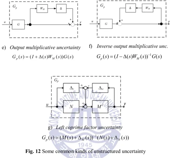
Uncertainty modeling
- Unstructured uncertainties
- Parametric uncertainties
- Structured uncertainties
- Linear fractional transformation
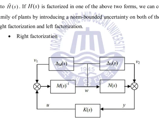
- Coprime factor uncertainty
For the purpose of initiating robust stability and robust performance theorems for the uncertainty of the left Coprime factor, we refer to the following definitions from (Lanzon and Papageorgiou, 2009). P PDÎR ´ with normalized graph symbols G% and GD and a denormalization factor RÎÃH¥ define the distance measure for the left Coprime factor uncertainty structure as implied by R as.
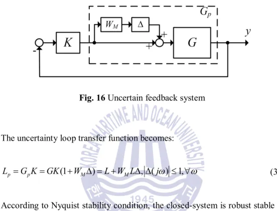
Stability criterion
- Small gain theorem
- Structured singular value ( ) m synthesis brief definition
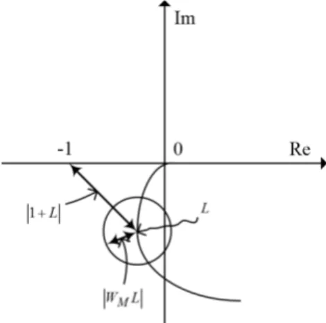
17, it can be seen that |1+L| is the distance from point -1 to the center of the disk representing Lp, and that |WML| is the radius of the disc.
Robustness analysis and controller design
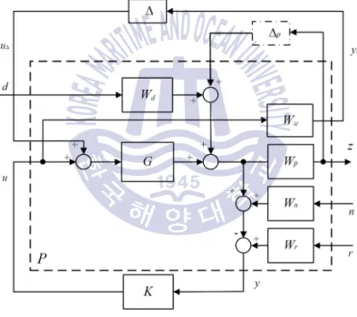
- Forming generalized plant and N - D ˆ structure
- Robustness analysis
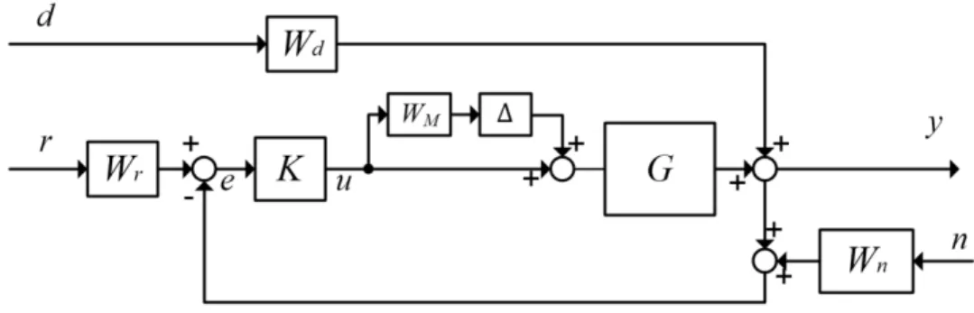
They can be constant or dynamic, describing the frequency content of set points, disturbances and noise signals. The system is internally stable if all transfer functions of the closed-loop system are stable, i.e. the rated capacity of the system depends on the sensitivity (So), which is a very good indicator of the ability to suppress interference.
To reduce noise, the one value of complementary sensitivity (To) in element N23i Eq. This implies that disturbances and noise reduction cannot be achieved in the same frequency range. Depending on the characteristics of disturbances and noise, disturbance suppression should be achieved in the low frequency range and noise reduction should be achieved in the high frequency range.
Robust controller using loop shaping design
- Stability robustness for a coprime factor plant description
After all initial weighting functions are in place, the DK iteration of the μ-synthesis toolbox in Matlab is applied to determine the The main design issue is choosing reasonable weighting functions W and WP. Inspired by frequency-shaped LQG synthesis, we shape the singular values of the open-loop response using weighting functions on the input and output of the system, creating a loop shape for which a stabilizing controller can be calculated. The uncertainty on the transfer M-1( )s is represented in inverse additive form (which is equivalent to representing the uncertainty on the M s( ) in direct additive form).
Reduced controller
- Truncation
- Residualization
- Balanced realization
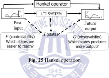
- Optimal Hankel norm approximation
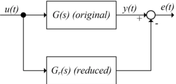
Find a reduced order model Gr(s) of degree k (McMillan degree) such that the infinity norm of the error. In general, there are three main methods to obtain a lower-order controller for a relatively high-order one: balanced truncation, balanced residualization, and optimal Hankel norm approximation. Then, if the eigenvalues are ordered such that |l1|<|l2|.., the fastest modes are removed from the model after truncation.
A balanced realization is an asymptotically stable minimal realization where the controllability and observability Gramians are equal and diagonal. The full model can then be reduced using balanced truncation, balanced residualization, or the optimal Hankel norm approximation. Let (A, B, C, D) be a balanced realization of G(s) with Hankel singular values rearranged to be a Gramian matrix.
Dynamical model of mobile rack vehicle
Dynamical model of longitudinal mobile rack vehicle
Furthermore, the force following the position input is approximately described as a first-order delay with a time delay. The linear expression of the force due to air resistance and friction is given by. where tmi is the time constant. The motor power can be obtained as. 93), the relationship between input and the motor force is given by.
Dynamical model of lateral mobile rack vehicle
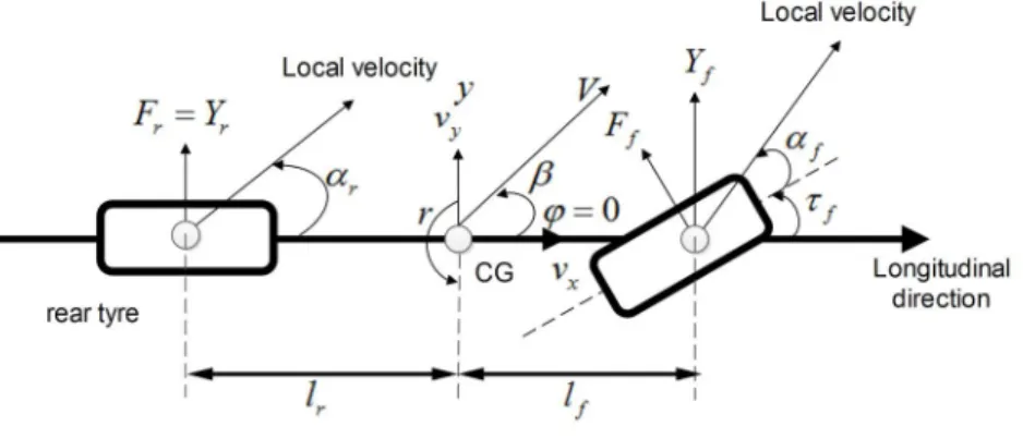
- Kinematics and dynamics of mobile rack vehicles
- Lateral vehicle model with nominal value
Parsing this term further shows that it is the sum of two terms; the lateral acceleration y&& and the centripetal acceleration Vj&. Then, the lateral force generated by the front and rear tires varies linearly with their slip angles (Rajamani R., 2006). The lateral deviation is the lateral deviation of the following mobile rack vehicle from the position of the target vehicle, and can be modeled as relationships between the states of the two vehicles.
It can be seen from the relation that the lateral deviation changes depending on the rotation of the following vehicle, as well as depending on the difference in the direction of movement of the two vehicles. Let D =g gL-gi-1 be the deviation, g j bi, ,i i lateral position, swing angle and slip angle of the ith MRV. 30 Open-loop system response for minimum maximum and nominal value: (a) Frequency responses of yaw angle; (b) lateral position frequency responses.
Controller design for mobile rack vehicle
Robust controller synthesis for longitudinal of mobile rack vehicles
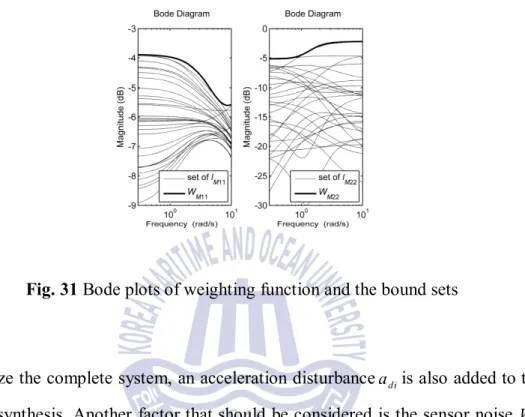
Recall that the weighting functions bound the entire radius lM (Skogestad and Postlethwaite, 2003) of the partial set of the plantG%i. The weighting uncertainty W sM( ) is also added to the system to combine with the input multiplier uncertainties DM( ) to create the perturbed plant. The complete control structure block is redrawn from the MRV connection block diagram to make it more general and easier to design the controller.
Furthermore, the complementary sensitivity function T0 should be small in high frequency range to reduce the effects of measurement noises on the controlled outputs as well as the control inputs. 35 represents the singular value plots of sensitivity S0 and complementary sensitivityT0, in which these results always satisfy the condition S s0( )+T s0( )= I at all frequencies. Then the weight performance Wp chosen as above is reasonable and satisfies the condition given in Eq.
Robust controller synthesis for lateral of mobile rack vehicles
- Lateral vehicle model with uncertainty description
- Controller design
- Robust performance problem
36 Stability and performance tests of the control system. stability, and ride comfort, over a wide range of parameter changes. The performance of the robust controller is then evaluated over the range of parameter variations by means of simulations. It is worth noting that the disturbance to D is normalized by the introduction of WM , which is the nominal distribution of the working range of the model.
The weighting matrix, which characterizes the input/output signals of the control system, must be formulated appropriately. At any frequency w, the magnitude of WM(jw) can be interpreted as the percentage of the model uncertainty at that frequency. Another factor to consider is the sensor noise Wn for the distance and communication measurements.
String stability of connected mobile rack vehicle
43 presents the single-valued graphs of sensitivity S0 and complementary sensitivity T0, in which these results always satisfy the condition. It is clear that the robust controller can successfully mitigate external disturbances and keep the complete system stable. L is defined as the transfer function from vehicle distance error to vehicle range error (i+1).
Clearly, the output range errors must be less than or equal to the input range errors to avoid propagating errors indefinitely along the connected vehicle string.
Lower order control synthesis
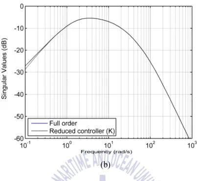
It is useful to reduce the system order as much as possible, which will simplify implementation and increase the reliability and maintainability of the system. 45Frequency responses of full-order (solid) and 3rd-order (dashed line) closed-loop system: (a) the singular value of channel 1 and (b) the singular value of. The corresponding plots are virtually identical, leading to comparable performance for the closed-loop systems.
In particular, the transient responses of the full-order closed-loop system and those of the reduced-order system are practically the same. 46, if the order of the system is further reduced to 2nd order or more, the performance will be greatly degraded. 46 Frequency response of full-order (solid) and 2nd-order (dashed) closed-loop system: (a) singular value of channel 1 and (b) singular value.
Numerical simulation and discussion
Mobile rack longitudinal control simulation and discussion
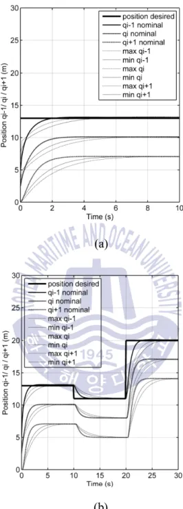
47Transient responses of MRV position due to single target and multiple targets: (a) single target, (b) multiple targets. Furthermore, there are only minor differences between the transient responses of the nominal, minimum, and maximum models. 47, the transient responses of mobile racks follow the lead vehicle without overshooting, the rising time less than three seconds.
48 Transient responses of MRV acceleration due to single target and multi-targets: (a) single target, (b) multi-target. 48, the acceleration responses of three-vehicle platoon are also illustrated which respectively follow the desired acceleration. 49 Transient responses of MRV velocity due to single target and multi-targets: (a) single target, (b) multi-target.
Mobile rack lateral control simulation and discussion
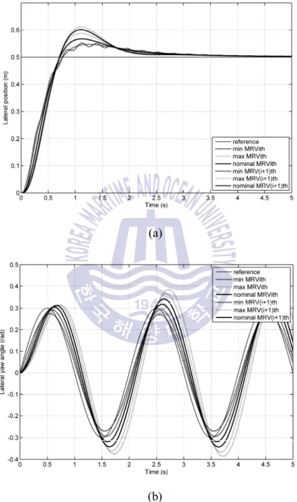
52The yaw angle response of the pack family of MRVs: (a) step responses of the yaw angle family, (b) sine responses of the yaw angle family. 53The lateral position response of the family of MRVs in the platoon: (a) Steering angle family with step input, (b) Lateral position family with step input. The lateral position responses of two MRVs in the platoon are also shown in the simulation as figure.
As a result, the lateral position family responses of two MRVs in a platoon are described. 54 Multi-target lateral responses of a family of MRVs in a platoon: (a) lateral position responses (b) Lateral control input signal. The capabilities of the control system of MRV lines under noise in the measurement signals are shown in fig.
Conclusion
On the other hand, the lateral control has performed stability of the yaw motion, such as the yaw angle family response and lateral position responses with step input and rectangular input. The lateral position responses of the family of MRVs have illustrated that the following MRVs can be behind the leading MRV with little overshoot.