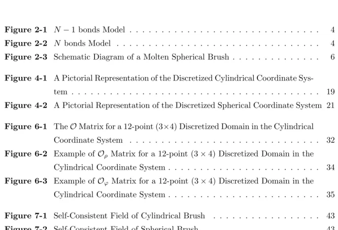
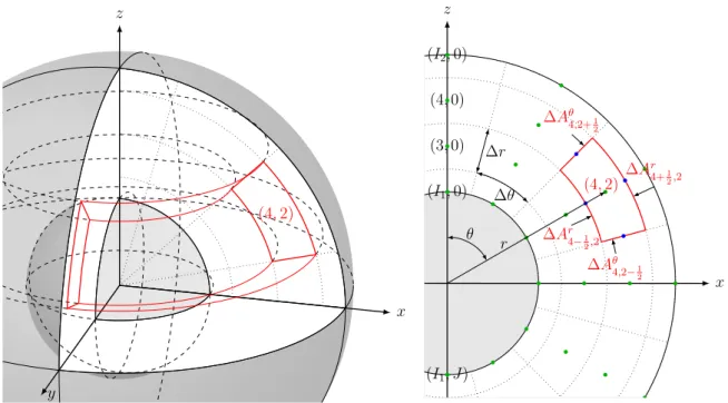
19 Figure 4-2 A pictorial representation of the discretized spherical coordinate system 21 Figure 6-1 TheOMatrix for a 12-point (3×4) discretized domain on the cylindrical. Recently, Matsenet al.[15] partially introduced the FVM in the spherical coordinate system in order to achieve better material conservation.
Molten Brush
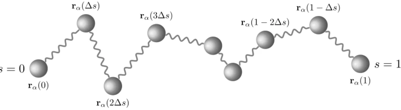
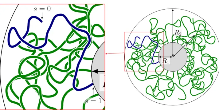
This entropic effect is often expressed by the strain energy of the chain whose Boltzmann factor corresponds to the Gaussian function. For the case of a cylindrical surface, I assume that the length of cylinder L is long enough to assume symmetry in that direction (z), so that the system can be completely specified by two variables, ρ and ϕ.
Self-Consistent Field Theory
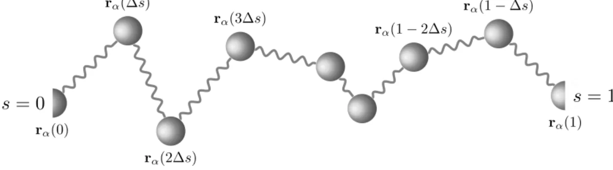
The product of the two partial partition functions is proportional to the probability that the sNth segment is at position r. Using the recurrence relation of the partition functions, the modified diffusion equations for the differential SCFT are obtained.
Spherical Coordinate System
We can remove this singularity and determine the first term of the right-hand side of equation (3.18) using the following method. One of the important properties of the modified diffusion equation is the existence of a field that, in principle, does not preserve the amount of material even in FVM; therefore, the preservation of SCFT material is an unsolved problem. However, the x3 coordinate is omitted in the position representation, r= (x1, x2), due to symmetry in the x3 direction.
Applying these results to equation (4.3), one obtains. 4.8) The result of the surface integral can be expressed as,. This process involves expanding the gradient of q(r, sn) using Taylor series, and subsequently evaluating the integral. Using this expression, one can finally convert equation (4.8) to a form corresponding to the 2D Crank-Nicolson equation.
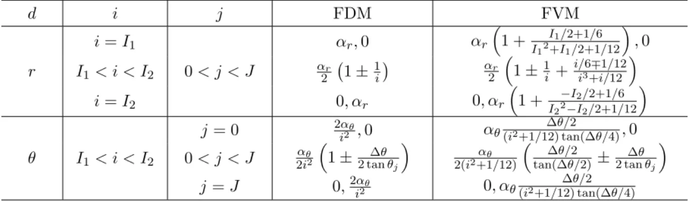
The symbolic form of the two equations is the same as in the FDM case, and I just need to analyze how δ2 ≡δ12+δ22 changes for the FVM case, as. The top surface of a cell Ci defined by ∆Ad. i+12eˆd is equal to the bottom area of the cell Ci+ˆed defined by ∆Ad. i+ˆed)−12ˆed, and the center of the top surface of cell Ci is also equal to that of the bottom surface of cellCi+ˆed, implyinghd+i =hdi+ˆ−e. Assuming that all q's are obtained by solving the FVM version of equation (4.13), one can check the material conservation in the following way.
Cylindrical Coordinate System
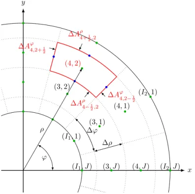
Each green dot represents a grid point (i, j), and the adjacent area surrounded by dotted gray lines indicates a grid cell Ci,j. Each blue dot indicates the center of the surface where the gradient calculation metric is selected. Only the ρ and ϕ directions are shown because there is no flux in the z direction due to the symmetry of the system.
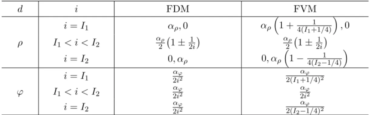
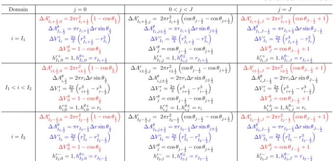
With the help of these equations, Bi,jd±, the geometric factors for the flux calculation, can be obtained. The above expressions are only accurate for the cells in the bulk of the system. For the cells at the system boundary, however, the interval of both the area and volume integral must be cut at the system boundary to calculate Bdi,j± as shown below.
For the polymer melt problem, the Neumann boundary is natural and no flow through the system boundary is expected, i.e. Note that for the side surfaces of the boundary cell, the metric must be taken at the center of the surfaces, hϕI1±,j =ρI1+1. We can now confirm that both in the bulk and at the boundary Bi,jρ± has no dependence on ϕ and are equivalent to the FVM formula for a one-dimensional cylindrical coordinate system.
Spherical Coordinate System
As in the case of cylindrical coordinates, it is necessary to discuss Bi,jd±at each boundary. For the spherical coordinate system, it is convenient to express the cell volume using a product of two independent components, ∆Vi,j = ∆Vri∆Vθj where ∆Vri = 2π3. The metric corresponding to these two surfaces must be taken at the center of the surfaces, hθI1±,j = rI1+1.
Using these expressions and the previously given ∆VI1,j values, the geometric factor BIθ1±,j can be calculated. The above process must be repeated at each boundary cell for the accurate implementation of FVM. For the rest of this section, their algebraic expressions, different from the non-boundary case, are presented.
If the cell Ci,j is at the corner of the domain (i=I1 ori=I2) and (j= 0 or j=J), for the correct calculation of Bdi,j± it is necessary to overlap the two corresponding recipes presented above; e. Mr. for the cell on the grafted surface of the south pole, apply the equations in examples 1) and 4) simultaneously. We can see that Bi,jr± have no dependence on θ and are equivalent to the FVM formula for a one-dimensional spherical coordinate system.
Comparison with Finite Difference Method
Cylindrical Coordinate System
Using FDM, derived in Chapter 3, each component of the two-dimensional Laplace value can be broadly calculated using equations (3.10) and (3.11).
Spherical Coordinate System
I have already explained that for FVM, the natural choice is the weighted sum of the cell volume as given in equation (4.22). The FDM formulation itself does not specify how the volume integral should be done, but considering the similarity of FDM and FVM, the simple integral method given in equation (4.22) will be used for FDM and will be the standard method when comparing material conservation . To calculate the segment concentration in cellCi, it is necessary to convert the direction integral into a summation.
The integral version of SCFT (equation (2.9)) and the Crank-Nicolson method (equation (4.4)) both suggest that their use is self-evident. The advantage of the bra-ket notation is that equation (6.5) is now written in the following simple algebraic form. For one direction of the proof, let me first assume that the material is conserved for the given numerical method.
In this case, the evolution matrix U is X(I − O)−1(I+O)X, assuming that I − O is invertible; so I need to check if the following matrix is symmetric. 6.24) Using the theorem in Appendix B, the X matrices in equation (6.24) are removable when checking for matrix symmetry. All the arguments I used from Equation (6.17) to Equation (6.22) are valid even when W = 0, so my FVM formulation preserves the amount of material when the 2D Crank-Nicolson method with operator division is used. By checking equation (6.22) for a few points, it is easy to confirm that material conservation is violated in FDM.
Alternating Direction Implicit Method
As a result, equation (6.27) reduces to the equation for one-dimensional Crank-Nicolson method without operator splitting. For the cylindrical coordinate system, FVM with the Crank-Nicolson method conserves material, thus FVM with ADI saves material ifW and. On the other hand, FDM with the Crank-Nicolson method does not conserve material for the cylindrical coordinate system, so there is no hope that two-dimensional FDM with the ADI method conserves material.
In this case, OdV−1 is symmetric for every d, because every equation confirming symmetry reduces to equation (6.22). Using the theorem in Appendix B, the twoX matrices in equation (6.33) are removable when checking for matrix symmetry. Using equation (6.35), V(I − Oρ)−1 is symmetric, and the second and third terms can be removed when checking the symmetry of the matrix.
In the previously formulated FVM in the cylindrical coordinate system, Bi,jϕ++Bi,jϕ−= αi2ϕ, which varies with respect to toi, and equation (6.43) cannot be satisfied; thus, even when using FVM with operator splitting, ADI method fails to preserve material. The case of the Cartesian coordinate system is somewhat more complicated because the FDM formulation can be equated to the FVM so that equation (6.22) is satisfied. When operator splitting is not used, the same logical steps are followed, one reaches equation (6.30) which cannot be satisfied with arbitrarily.
![Figure 6-3: Example of O ϕ matrix for a 12-point (3 × 4) discretized domain in the cylindrical coordinate system, i ∈ [2, 4] and j ∈ [1, 4]](https://thumb-ap.123doks.com/thumbv2/123dokinfo/10535870.0/45.892.109.823.115.278/figure-example-matrix-point-discretized-domain-cylindrical-coordinate.webp)
Douglas-Gunn Method
To verify that FVM preserves material, it is necessary to check whether the following matrix is symmetric when Oϕ and Oρ are taken for FVM. Using the theorem in Appendix B, the matrices in equation (6.54) are removable and I only need to check the symmetry of the following matrix. The last expression is equivalent to equation (6.36) and all remaining stories in the previous section can be shared.
It means that the material conservation fails in the cylindrical and spherical coordinate system, while the Cartesian coordinate system has the ability to preserve the material quantity, when using the FVM method with Douglas-Gunn operator division. Because the material conservation for the Douglas-Gunn method is exactly the same as the ADI case, the two cases share the same column in Table 8-1.
Pseudo-spectral Method
For the initiation of the pseudo-spectral method, the Strang partition is applied to the modified diffusion equation. Now, by repeating the processes from equation (6.1) to equation (6.13) with the standard complex version of the bracket notation, it is straightforward to show that the actual material conservation condition is that VU be Hermitian. The separation operator did not affect the preservation of the material in this one-dimensional case, but its effect is somewhat complicated.
The FVM is designed and known to perform better, but the material conservation of the modified diffusion equation is not equivalent to the material conservation of normal diffusion equation because the segment volume of SCFT is obtained by integrating products of two partial partition functions over space. In this research, to prove the usefulness of FVM in the SCFT, I successfully developed an algebraic test using bracket notation that verifies the material conservation of each numerical method. The material conservation condition was equivalent to the condition that the product of volume matrix and the evolution matrix is symmetric, VU = (VU)T.
Applying the same algebraic test to the alternating direction implicit (ADI) method and the Douglas-Gunn method, I show that the FVM in the cylindrical and spherical coordinate systems cannot generally save material, but careful numerical tests show that , depending on the problem, using FVM can still improve the material conservation compared to the FDM case. A possible suggestion is to calculate the standard of VU −(VU)T and find its effect on material preservation. The material conservation test presented in this thesis is very versatile and its application to the pseudo-spectral method was also possible.
![Figure 6-1: The O matrix for a 12-point (3 × 4) discretized domain in the cylindrical coordinate system, i ∈ [2, 4] and j ∈ [1, 4]](https://thumb-ap.123doks.com/thumbv2/123dokinfo/10535870.0/42.892.247.755.194.303/figure-o-matrix-point-discretized-domain-cylindrical-coordinate.webp)
