The primary objective of the study is to evaluate the classification results on a subset of the Places365 dataset after applying different clustering algorithms during the preprocessing phase. Through a series of experiments, we show that the choice of clustering algorithm significantly affects the performance of the classification model. I would like to express my sincere appreciation to my thesis advisor, Professor Martin Lukac, for his invaluable mentorship and unwavering motivation throughout every phase of the project.
The primary aim of this thesis is to investigate the influence of three separate clustering techniques on the performance and outcomes of a classification model applied to an autonomously generated data set. Specifically, this study will analyze the classification results of the widely used Convolutional Neural Network (CNN) model, AlexNet, after using various clustering algorithms. By evaluating the classification performance of the AlexNet model following the application of three separate clustering techniques to an autonomously generated dataset, this thesis hopes to provide valuable insights for the future works.
Clustering Algorithms
Similarity-Based Clustering
Afterwards, k-means then reassigns all data points to their nearest centroids and recalculates the centers of the newly formed clusters [16]. The most commonly used criterion is to minimize the squared error, which is the sum of the squared Euclidean distances between data points and their nearest cluster centroids.
Density-Based Clustering
The algorithm is widely used in various fields, including environmental monitoring, bioinformatics, and image processing.
Model-Based Clustering
Image Classification
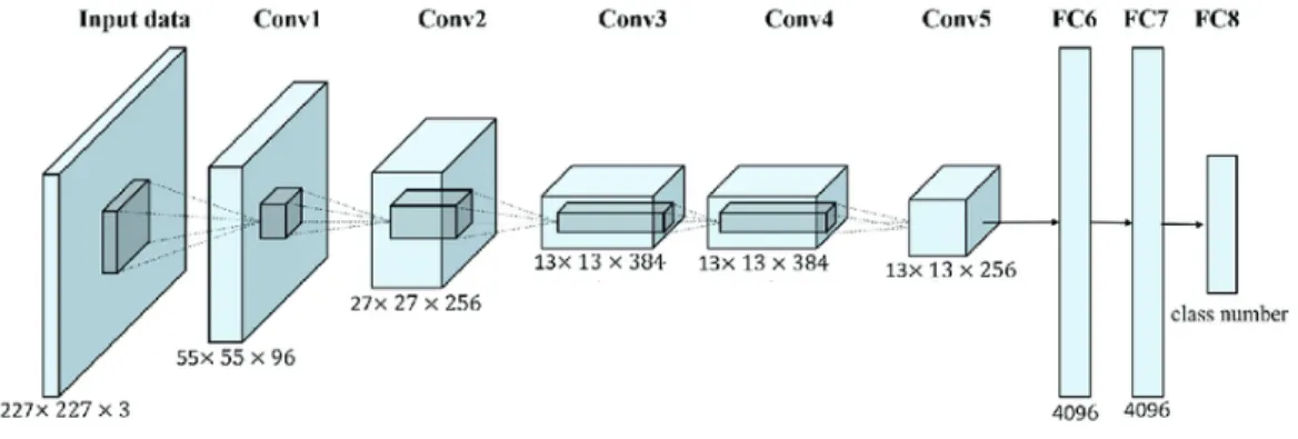
Alexnet
It is a deep CNN architecture that marked a turning point in the field of image classification by demonstrating the potential of deep learning for image recognition tasks. After its success in the ILSVRC, AlexNet became a fundamental architecture for numerous image classification tasks and stimulated further research into deep learning for computer vision. AlexNet has been applied in various domains, such as medical image analysis [25], remote sensing [26], and object detection [27].
The specific choice of the data set is not decisive for the research objectives and findings; rather, it serves as a representative sample to explore the algorithms and methodologies used in the study. Places is a large-scale image dataset and there are different variations of the dataset depending on its size. For this project, all the experiments were done using the images from the Places365-Standard version.
The Places365 standard is a subset of the Places dataset with over 1.8 million images for training [31]. All the images from the dataset are of good quality and colored with a resolution of 256x256 pixels [31]. It has been used in various research studies and competitions, such as the Places Challenge, which is a competition for scene recognition algorithms [31].
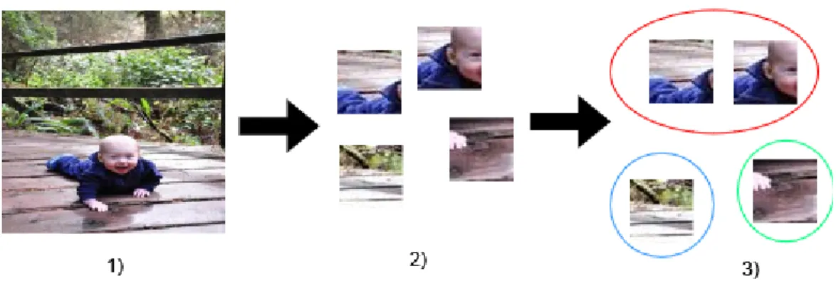
For the scope of the project, 145,000 images were randomly selected and downloaded from the dataset. For each image, four non-overlapping samples with a resolution of 40x40 pixels are extracted and included in the training set.

Experimental Structure
- Clustering
- Classification
- Performance Evaluation
- Accuracy
The differentiating factor of DBSCAN is that during the initialization of the clustering method, the value of epsilon (eps) is used instead of the number of clusters. This ensures that the integrity of the dataset distributions is maintained for subsequent analysis and evaluation. Before the final phase of the experiments, data transformation is performed to ensure that the input data is in the correct format for the CNN model.
For the purpose of the experiment, the last layer of the model is modified from the initial 1000 classes [22] to the values of N used therein. During the training of the model, the epoch was set to 50 with a batch size of 32. In the case where the loss value does not change on the validation set for 10 consecutive epochs, the training is terminated and the last state of the model with the best performance is saved.
To compare the performance of the mentioned model, two commonly used evaluation metrics for classification tasks are used: classification accuracy and Negative log-likelihood loss (NLLLoss). Accuracy measures the proportion of correctly classified images out of the total number of images. It will be evaluated during different phases of the classification and for each class during the test phase.
Negative log-likelihood loss (NLLLoss) is an evaluation metric commonly used in the context of classification problems, especially in the field of deep learning. In this formula, N represents the number of samples in the data set, 𝑦𝑖 is the true class label for the i-th sample, and 𝑝(𝑦𝑖) is the predicted probability for that class.
Setup
- Hardware
- Software and Data
- K-Means
- DBSCAN
- GMM
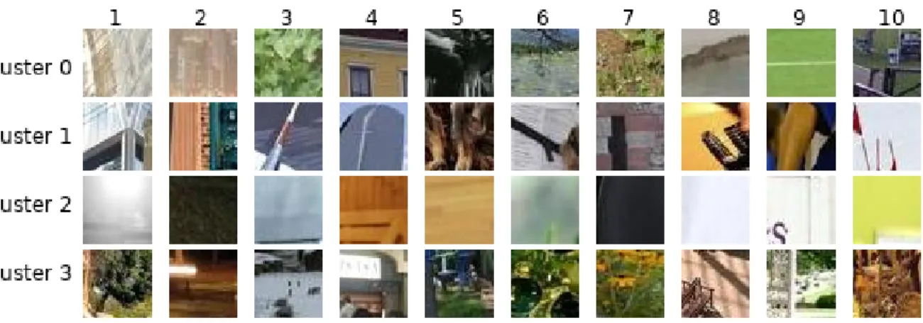
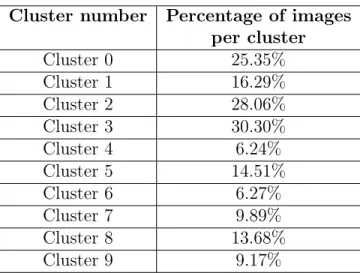
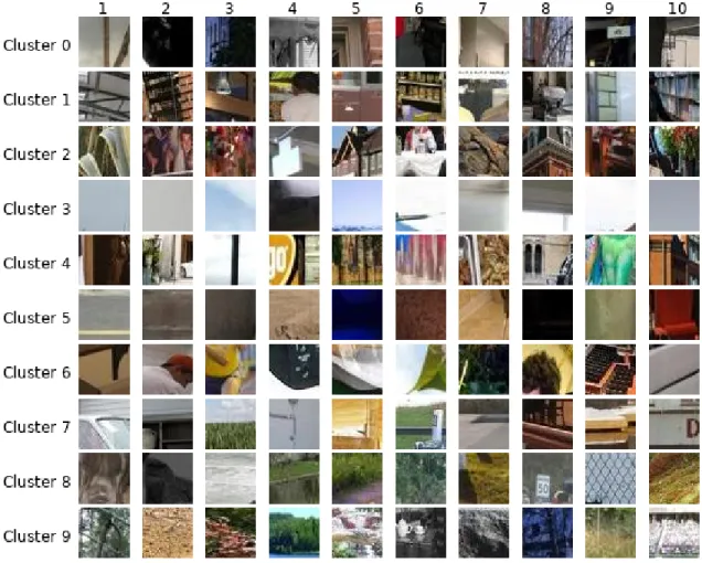
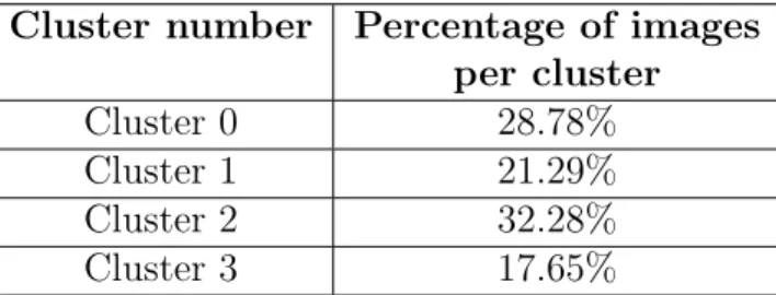
The notable observation here is the relatively balanced distribution of images between the clusters, as no single group appears to be strongly dominant. For a better understanding of K-Means clustering results, 10 randomly selected images per cluster has been demonstrated in Figure 4-1. In this scenario, there is a greater variation in the percentage of images assigned to each cluster.
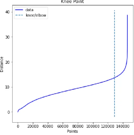
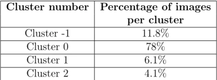
The plot shown in Figure 4-3 was obtained using the NearestNeighbors method from the scikit-learn library [33]. Using the elbow method implemented in the KneeLocator Python library, an eps value of 13.68 was calculated. By examining the data distribution, it becomes clear that the algorithm has categorized a significant portion of images into a single category.
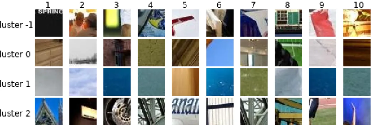
Finally, Cluster 2 consists mainly of images containing distinct objects, such as building tips, brake discs, aircraft, and steel bars. Similar to previous clustering algorithms, Figure 4-5 presents distinct visual patterns among the Gaussian Mixture Model (GMM) clustering results. Similar to the K-means clustering results, Table 4.5 also shows image segmentation with the number of components set to ten.
The examples shown in Figure 4-6 allow us to see some patterns between the clusters. Group 1, on the other hand, is likely to consist of images that highlight watersheds or significant changes in feature values.
Classification
K-Means
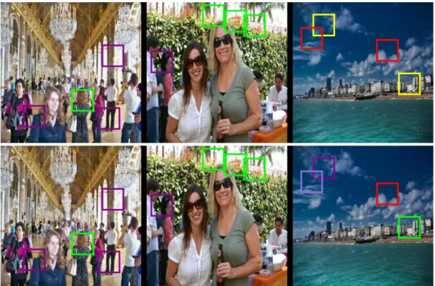
The top image in Figure 4-8 presents a selection of results from the K-means clustering algorithm. In the second image, we observe a discernible pattern in Group 3, represented by the red color, as it groups together images containing leaves. However, in the first image, the group also includes a photo that mainly features a woman's hair.
Therefore, it is likely that Cluster 3 includes images with wavy lines, as evidenced by the presence of another image in the second example, which similarly shows a woman's hair. Based on the first and second images, it appears to group images that contain straight lines and potentially darker shades. In contrast, cluster 2, represented by lime-colored contours, presents three accurate predictions out of three.
Following the patterns observed in the other two clusters, cluster 2 may include uncertain forms such as clouds or mostly. However, due to its presence only in the third image, there are fewer examples available to confirm this hypothesis with certainty. The bottom image in Figure 4-8 shows the same images, but after using AlexNet to classify partitions into classes.
DBSCAN
We can see from the examples in Figure 4-9 that the clustering algorithm and model mostly grouped partitions into a single class.
GMM
The model showed a classification accuracy of 74.87% and 66.8% on the test dataset for the respective configurations. The first part of Figure 4-10 shows that the Gaussian mixed models algorithm made different decisions compared to other clustering techniques. Nevertheless, it successfully differentiated the building in the third image from the other images within the "Dark Magenta" cluster.
Furthermore, the algorithm maintained consistency with the “wavy and hair” pattern of Cluster 2 by including the sample from the top portion of the second image in the cluster. Given these results and from Table 4.8, there is a good chance that the model was able to learn some patterns from clusters, and especially from lime and dark magenta groups. Upon closer inspection, it was able to separate the buildings from the rest, but still in the wrong cluster.
Results comparison
The most plausible explanation for this discrepancy is the model's inability to learn effectively due to the substantial imbalance in class sizes within the dataset, noted in Table 4.3. In conclusion, this thesis examined the impact of different clustering algorithms - K-Means, DBSCAN and Gaussian Mixture Models - on the performance of a supervised classification model, specifically AlexNet. Through a series of experiments, we found that the choice of clustering algorithm has a substantial impact on the performance of the classification model.
The models trained on datasets created after applying Gaussian mixture models and K-means showed significantly high classification accuracy, while DBSCAN case produced poorer outcomes due to insufficient clustering of the images. For future research, it would be valuable to investigate other clustering algorithms and their effects on various classification models. In addition, investigating the use of ensemble methods that combine the strengths of multiple clustering algorithms may lead to further improvements in classification accuracy.
Finally, exploring the impact of feature extraction and dimensionality reduction techniques on the performance of clustering algorithms would contribute to a more nuanced understanding. Lim, “Hierarchical text classification and evaluation,” in Proceedings 2001 IEEE International Conference on Data Mining, p. Intelligent Robots and Systems (IROS), p.
Kai-fei, “Improved search for initial centers of k-means clusters,” in 2015 Ninth International Conference on the Frontier of Computer Science and Technology, p. Sarasvady, “Dbscan: Past, Present and Future,” in Fifth International Conference on Applications of Digital Information and Internet Technologies (ICADIWT 2014), p.
Image distribution per cluster. K-Means for 4 clusters
Image distribution per cluster. K-Means for 10 clusters
Image distribution per cluster. DBSCAN with eps=13.68
Image distribution per cluster. GMM for 4 clusters
Image distribution per cluster. GMM for 10 clusters
Classification Results. Loss and Accuracy for K-Means during training,
Classification Results. Loss and Accuracy for DBSCAN during train-
Classification Results. Loss and Accuracy for GMM during training,
Classification Results. Accuracy and NLLLoss score for three algo-
Classification Results. Accuracy by class for three algorithms during