SENet with 3 Hidden Layers Plus Fallout Layers 120 4.39 Third Fold Confusion Matrix Training for (a). SENet with 3 Hidden Layers Plus Fallout Layers 128 4.45 Fifth Fold Confusion Matrix Training for (a).
Background
Although it may be a simple task, it demonstrated the effectiveness of deep learning applications on medical images. All in all, detection and classification using deep learning is becoming more common in the medical field.
Problem Statements
Aims and Objectives
Leukemia
- Acute Lymphocytic Leukemia
- Acute Myelogenous Leukemia
- Chronic Lymphocytic Leukemia
- Chronic Myelogenous Leukemia
Acute lymphocytic leukemia (ALL) is a type of leukemia that is mostly seen in young children, but it can also occur in adults (Shaheen, et al., 2021). This development can be observed in 3 different phases: the chronic phase, accelerated phase and explosive phase (Bibi, et al., 2020).
Detection and Classification
In the chronic phase, the leukemia is still developing, and there may be no symptoms or mild symptoms such as fatigue and a slight weight loss. For the second phase, which is the accelerated phase, symptoms may be more obvious, such as increased fatigue, weight loss, and a swollen stomach caused by an enlarged spleen.
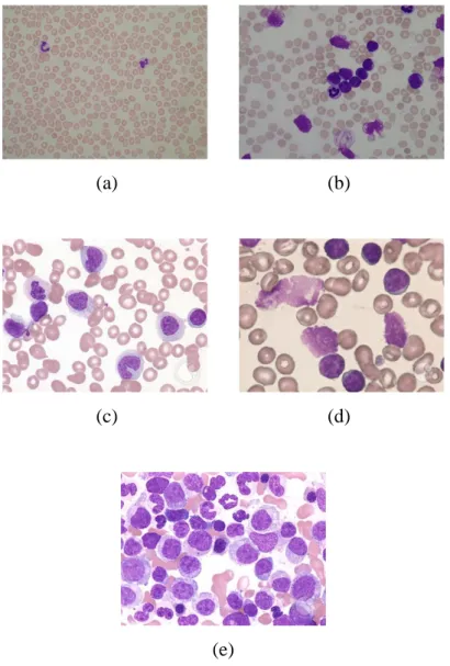
Morphology of Leukemia and Peripheral Blood Smear Findings
In addition, in CLL, smear cells can be observed in the peripheral blood smears, as neoplastic cells are fragile and may smear during slide preparation. Finally, the findings regarding the peripheral blood smear of CML are that it has left shift leukocytosis.
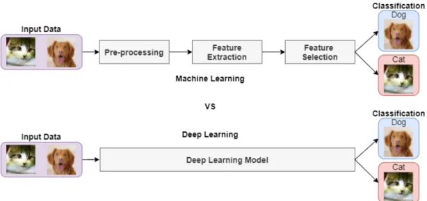
Deep Learning
- Deep Supervised Learning
- Deep Unsupervised Learning
- Deep Reinforcement Learning
- Deep Semi-supervised Learning
- Deep Transfer Learning
However, it may take more time and computing power to achieve this in a larger workspace (Alzubaidi, et al., 2021). One application of deep semi-supervised learning can be seen in classification tasks regarding text documents (Alzubaidi, et al., 2021).
Types of Artificial Neural Networks
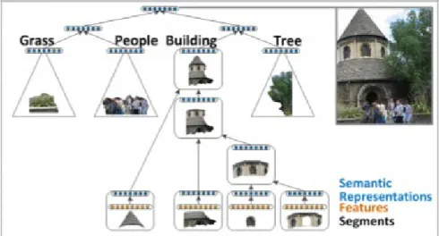
Recursive Neural Network
There are two types of approaches to perform transfer learning using pre-trained models: feature extraction and fine-tuning. As a result, an RvNN tree structure is implicitly created for each merge decision, with the final output being the full scene image, which is said to be the root of the structure (Alzubaidi, et al., 2021).
Recurrent Neural Network
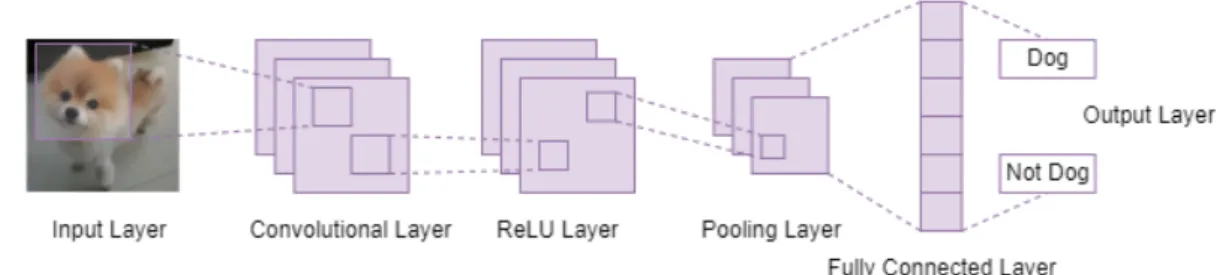
Convolutional Neural Network
In addition, CNNs allow large-scale networks to be implemented more easily compared to other types of neural networks (Alzubaidi, et al., 2021). Therefore, due to the exceptional performance that CNNs can provide, it is currently widely adopted in multiple applications such as face detection, object detection, image classification, facial expression recognition, speech recognition, and so on (Indolia, et al., 2019).
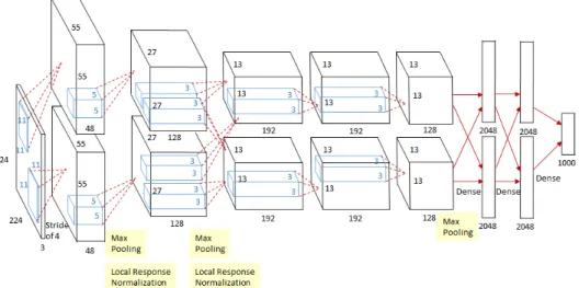
CNN Architecture
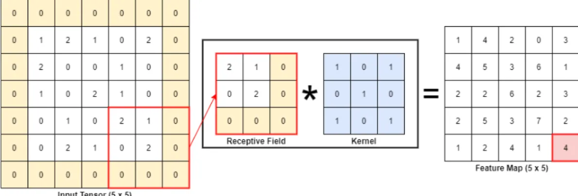
- Convolution Layer
- Pooling Layer
- Activation Function
- Batch Normalization
- Dropout
- Fully Connected Layer
However, a larger step can also be used to achieve feature map undersampling (Yamashita, et al., 2018). 0,𝑥𝑥< 0 (2.4) The curve of the ReLU function and its derivative is illustrated in the figure below.
Types of CNN Architectures
- AlexNet
- ZFNet
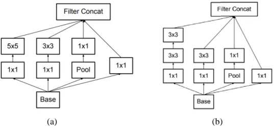
- GoogLeNet
- ResNet
- ResNeXt
- SENet
- DenseNet
The fully connected layer is often found at the end of a CNN architecture (Alzubaidi, et al., 2021). Moreover, auxiliary classifications are also implemented to improve the convergence speed of the network (Khan, et al., 2020).
Performance Metrics
- Accuracy
- Precision
- Recall
- F1-score
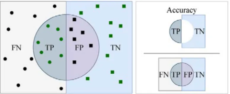
- Confusion Matrix
- ROC Curve
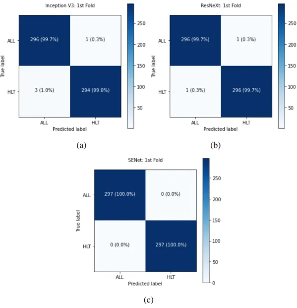
As shown in Equation 2.8, precision measures the number of true positives for all data where data the model labels as positive. All predictions made by the model are plotted on the confusion matrix, allowing better visualization of performance. The diagonal elements of the confusion matrix are known as the true positives or true negatives.
The other elements of the confusion matrix are known as false positives or false negatives. The area under the ROC curve (AUC-ROC) then measures the degree of the model's class separability for each class.
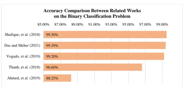
Related Works
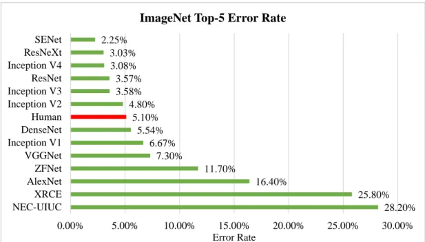
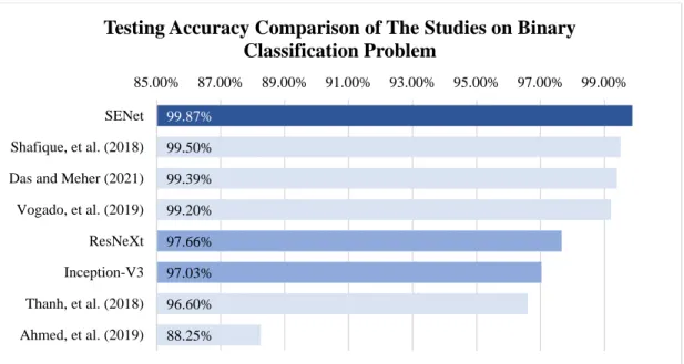
Meher (2021), in which the MobileNetV2 and ResNet18 models are hybridized into one model, and the transfer learning technique is also used in the training process. As a result, the proposed hybrid model is able to achieve an accuracy of 99.39% in the binary classification problem. Overall, the deep learning approaches used in leukemia detection and classification and their accuracies are summarized and illustrated in the bar graphs shown below.
In the studies discussed earlier, most models are trained using microscopic samples primarily from the Acute Lymphoblastic Leukemia Database (ALL-IDB) (Scotti, Labati, & Piuri, 2011). In addition, most of the literature also faces a lack of samples available for training and testing.
Project Flow
Project Requirements
- Hardware Requirements
- Software Requirements
- Programming Language Used
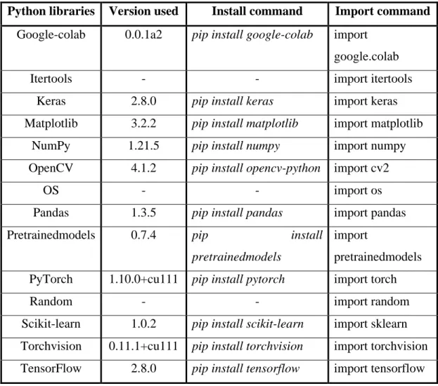
- Open-Source Libraries
The software used is an Internet browser that allows the use of two websites called Google Colab and Google Drive for the purpose of training DL models. Google Colab is an online environment that makes it possible to execute code in the browser or more specifically in the cloud. On the other hand, Google Drive is an online service that provides cloud storage for all kinds of files and folders.
Python Libraries Version Used Install Command Import Command Google-colab 0.0.1a2 pip install google-colab import. Scikit-leer 1.0.2 pip install scikit-leer import sklearn Torchvision 0.11.1+cu111 pip install torchvision import torchvision TensorFlow 2.8.0 pip install tensorflow import tensorflow.
Dataset Acquisition
Dataset Splitting
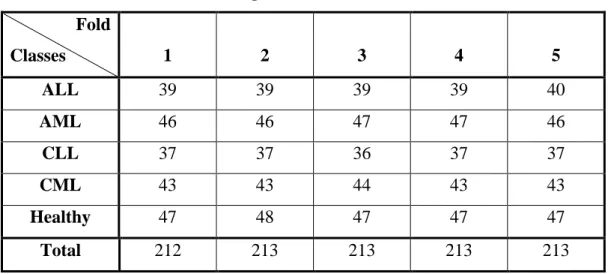
Next, to ensure that the models will not be tested with images used for training, the training and test set will be separated between the dataset. This is done using the 'KFold' class of scikit-learn library which divides the dataset into k folds of train and test sets, in which this project, a k of 5 is implemented. To maintain a balanced class distribution in the datasets, the stratified k-fold cross-validator, which is the 'StratifiedKFold' class, will be used instead of the 'KFold' class.
With that said, the dataset for binary and 5-class classification problems is divided into each fold as shown in Tables 3.3 and 3.4. It is noted that the data set is divided for each fold based on the 80/20 rule where the training set consists of 80%.
Dataset Augmentation
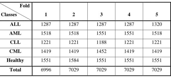
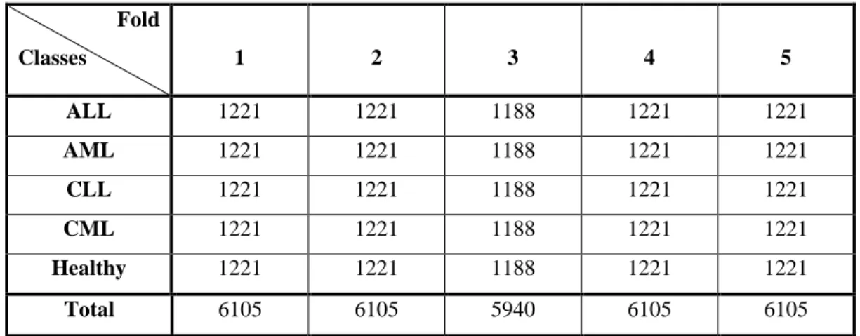
On the other hand, Figure 3.2e is the resulting image after a 40% height shift, while Figure 3.2f is the resulting image after a 40% width shift. Furthermore, Figure 3.2g is the resulting image after flipping vertically, while Figure 3.2h is the resulting image after flipping horizontally. Hence, after the image transformations, each image sample is increased by a factor of 33, effectively increasing the overall data set for each class.
The code for this segment is listed in Code Listing 5 of Appendix A, and the new number of samples for each class and its source is tabulated as shown in Tables 3.5 and 3.6. The bar graph shown in Figure 3.3 illustrates how the data set for each fold is allocated.
Model Training
Once the models are set up, they will be trained on a pre-processed data set split for each fold. Starting with a binary classification problem, the final layer will have 2 nodes and a sigmoid activation function will be used as the classifier. In addition, binary cross-entropy will be used as the loss function, ADAM as the optimizer, and accuracy as the evaluation metric.
On the other hand, the last layer will instead have 5 nodes for the 5-class classification problem, and the softmax activation function will be used as the classifier. In addition, categorical cross entropy will be used instead of binary cross entropy, while the loss function and evaluation statistics remain the same.
Model Evaluation
The number of epochs for training the binary classification problem will be set to 10, while when training the 5-class classification problem, it will be set to 25. In each epoch, the models with the highest validation accuracy will be kept as the models final, while those lower than the previous highest values will be ignored.
Model Improvement
This phenomenon happens when the model underfits the data, leading to the poor performance on the training data, which also leads to a high error on the unseen test data. One of the ways to lower the bias of a model is to train a model with a larger and more complex network, or to train the model long enough to learn the important features of the data . On the other hand, variance is the variability of the model in making predictions, such that it measures how many adjustments the model can make based on the given data.
This phenomenon occurs when the model overfits the data, where the model shows a good performance on the training data, but a high error is observed on the unseen test data. To lower the variance of a model, more data should be used to train the model, or implement regularization in the model (Wickramasinghe, 2021).
Project Costs
Project Management
Fold 1
Fold 2
Fold 3
Fold 4
Fold 5
Fold 1
Fold 2
Fold 3
Fold 4
Fold 5
Fine-tuned SENet Models
- Fold 1
- Fold 2
- Fold 3
- Fold 4
- Fold 5
Binary Classification Problem for SENet with 3 Hidden Layers Plus Dropout Layers
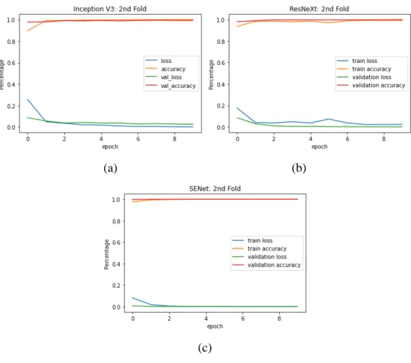
- Accuracy and Loss Against Number of Epochs
- Precision, Recall, and F1-score for Leukemia Subtypes Classification
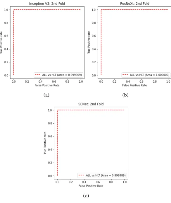
- ROC Curve
- Confusion Matrix
Discussion
The bar graph shown in Figure 4.53 compares the mean precision, recall and F1 score between SENet model A and B. In addition, the model is also unable to measure the mean precision, recall and F1 score for all classes of the SENet model A. The bar graph shown in Figure 4.55 compares the mean precision, recall and F1 score between SENet model A and C.
It is observed that the average testing accuracy for SENet C model C increases by 0.52% compared to SENet model A. The bar chart shown in Figure 4.57 compares the mean precision, recall and F1 score between SENet model A. and D.
Project Review
Project Findings
It is clear that the SENet model encountered the problem of binary and 5-class classification compared to other models. The SENet C model also had a small improvement in class separation compared to the SENet A model. Additionally, the SENet D model saw an improvement in precision, recall, and F1 score for most classes compared to the SENet A model.
The ROC curves, AUC-ROC values and confusion matrices also show that the SENet model D has a stronger class separation for all classes. Small improvements are observed in terms of precision, but the model has a slightly lower recall and F1 score than the SENet model A.
Recommendations for Future Improvements
For example, the ALL class can be further categorized into 3 subtypes: ALL-L1, ALL-L2 and ALL-L3. Therefore, it is recommended that these subtypes be included in future projects so that a more specific prediction can be made, enabling effective and accurate treatment of the types of leukemia detected and classified.
Conclusion
Detection of acute lymphoblastic leukemia and classification of its subtypes using pretrained deep convolutional neural networks. Listing A.20: Testing the Inception-V3 model for binary and 5-class classification problems with unseen test data.