Mt Maintenance costs of the CPV systems for t year ($) Ot Operating costs of the CPV systems for t year ($) S Incident solar rays. St Annual rated energy output of the CPV systems for t year (kWh) ST Solar tracking.
Problem statement and research objectives
To develop a computational algorithm to simulate mutual shading between dual-axis CPV sun tracking system in different field layout designs. To evaluate the shadow effect on a dual CPV sun tracking system considering different field layout designs.
Scope of research
This research will greatly benefit our society as it can help improve our technologies for more efficient use of renewable energy.
Outline of thesis
LCOE is described as the price per produced unit of energy over the entire lifetime of the system. One of the plans to lower the LCOE is to increase the power generated by the PV/CPV system.
Importance of sun-tracking (ST) system
Types of sun-tracking (ST) system
In general, each type of 1-axis ST system has the following basic characteristics as listed in Table 2.1. The main advantage of this type of ST system is that it can be installed densely together in a limited area. This type of ST system is typically used in high latitude locations because the position of the sun does not become as high at noon (Johnson-Hoyte et al., undated).
The main function of this ST system is to change the tilt angle according to the path of the sun.
Justification of both the sun-tracking (ST) system
Components 1 axis ST system 2 axis ST system
Basic computations of sun position
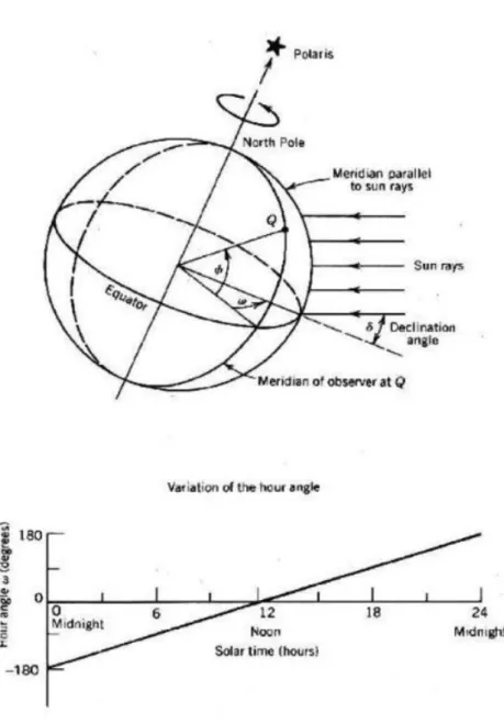
Normally, the LCT can be used to calculate the solar time of the specific location. The hour angle, ω, basically describes the difference between the time of the current day and its solar noon (Dawson, 2013). In the previous part of Section 2.1 it is mentioned that the GF can help improve the accuracy of any type of ST system either 1-axis (e.g. polar ST system) or 2-axis ST system (e.g. azimuth-elevation ST- system) to increase.
According to Chong and Wong (Chong and Wong, 2010), calculations or calculations of the sun's position can be done by setting the 3 important parameters and applying the corresponding values to the corresponding equations derived from them.
Overall review of the electrical performance of PV/CPV system
He outlined that the electrical power generation of a 2-axis tracking PV system was a 43.87% improvement over that of a fixed-mount PV system with a 32° slope facing south. Based on the aforementioned studies, it is deduced that the ST PV system has a large electrical performance improvement over the fixed-mount PV system. However, no studies have been done on the optical loss of the dual-axis sun-tracking PV system field.
Land costs may fall within annual operation and maintenance costs or initial investment, depending on land ownership.
Methods/Algorithm used by researchers on layout optimization
- Geometry of mutual shadowing
- Ray-tracing (point-to-point) method
- Ray/Plane algorithm (Four-point method)
Dähler, Ambrosetti and Steinfeld, 2017) also made a simulation model in 2017 using the ray-tracing method under two assumptions, i.e. (GCR). In their study, the whole tile is assumed to be completely shaded provided as long as the central point of the tile is shaded.
A special algorithm can be used to significantly reduce the computation time of the ray-tracing method.
Research approach in the optimization of large solar power plant
Based on the research conducted by Pons and Dugan (Pons and Dugan, 1984), they mentioned that the edge effect can be neglected in square or near-square array layout configurations, provided that the layout configurations had more than 50 collectors. The many other research groups have neglected these edge or boundary effects in their studies. Dähler, Ambrosetti and Steinfeld, 2017) that the optical performance of a solar dish field can be optimized in terms of shading efficiency and ground cover.
In addition, they also mentioned that the boundary effect has been excluded in their study, as this effect is assumed to be less important as the field size increases.
Levelized cost of electricity (LCOE)
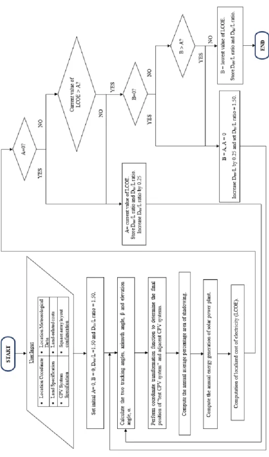
According to the previous work done by other researchers, the optimization of PV field layout design only comes with the consideration of the system performance by reducing or eliminating the mutual shading between the PV system. In this research, a new calculation algorithm is proposed to optimize the LCOE of the field layout design according to the local meteorological data. The methodologies of the simulation algorithm to optimize both the square array and staggered array layout configurations are shown in Figure 3.1 and Figure 3.2, respectively.
Thus, a study of the economic balance between land-related costs and electricity generation costs is carried out using simulated results.
Sun-tracking (ST) angles
Coordinate transformation
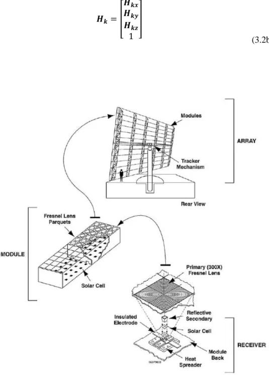
4, where the local origin, C(0,0,0), is located at the center of the structural frame of the CPV system instead of at the center point of the CPV field. There are four corners of the CPV system, with each corner represented by an edge point. The final coordinate of the structural frame of the CPV system is defined as C (𝐻𝑐𝑥, 𝐻𝑐𝑦, 𝐻𝑐𝑧) after performing the coordinate transformation.
To transform the position of the CPV system structural frame from the origin of the global coordinate system to the final coordinate, a translational transformation method is essential to transform the position using coordinate transformation.
The Sun-incident ray and ray/plane algorithm
Levelized cost of electricity (LCOE)
The lowest possible calculated value of LCOE for the CPV system in solar power plant should be selected to determine the optimized layout design.
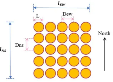
Layout configuration
The lowest possible calculated value of LCOE for the CPV system in solar power plant should be selected to determine the optimized layout design. where T is the life of the project in years, t is the number of years, It is the initial capital cost of the CPV systems including construction, installation, hardware and software of control system etc., Mt is the maintenance cost of the CPV systems for t year,. Ot is the operating cost of the CPV systems for t year, Ft. is the interest expenses of the CPV systems for t years, r is the discounted rate of the CPV systems for t years, St is the annual rated energy output of the CPV systems for t years. and d is the degradation rate of the CPV systems. between the CPV systems in east-west direction to the dimension of a solar collector), Dns/L ratio (the ratio of spacing distance between the CPV systems in north-south direction to the dimension of a solar collector) and spacing angle, θ , has been suggested. The ground cover ratio (GCR) was also implemented in the research as the ratio of the total area of the GPV system to the total area of land.
In the simulation of the layout of the scaled arrays, the positions of the CPV systems in the solar power plant are shown in Figure 3.8.
Annual energy generation
Optimization studies for both square array configuration and staggered array configuration were conducted in a city located in the north of Borneo Island, Kota Kinabalu, Malaysia, considering local meteorological data, shading efficiency, annual yield of energy, LCOE, land leasing cost, land aspect ratio (LAR) and the advantage effect.
Shadowing
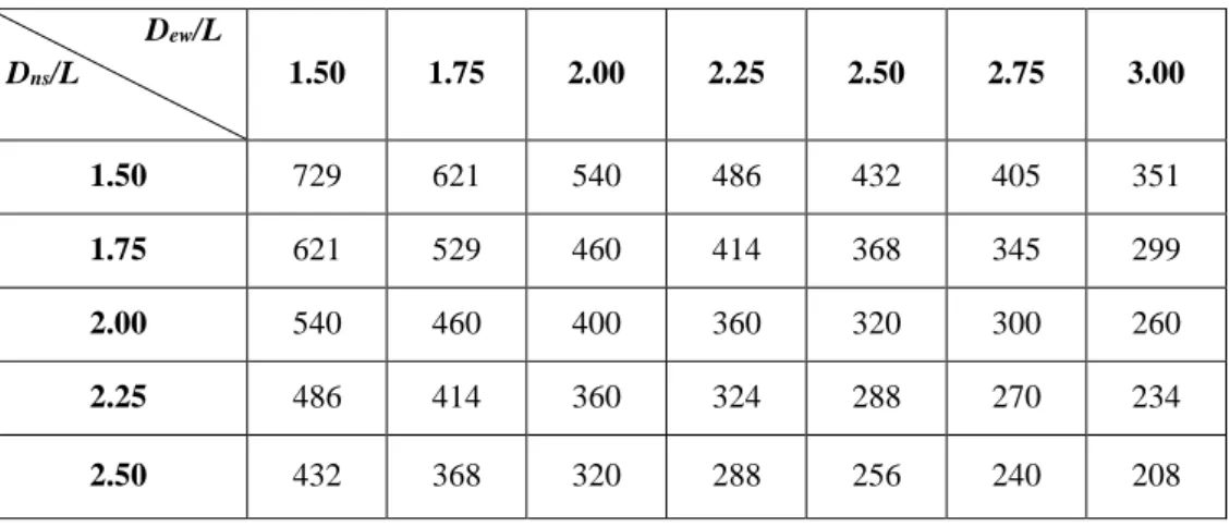
This minimum value is set to avoid a possible collision between any two CPV systems. The maximum possible number of CPV systems to be allocated to a given land area of 62,500 m2 is calculated for both the square array and staggered array layout configurations in Table 4.1 and Table 4.2, respectively. The simulation result also shows that the distance between two adjacent CPV systems in the east-west (E-W) direction has a greater influence on the shading effect compared to that in the north-south (N-J) direction.
The results were taken from the minimum Dou/L ratio for each angle to avoid collision between adjacent CPV systems.
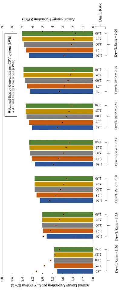
Annual energy generation
The annual energy output for each CPV system is directly proportional to the Dew/L and Dns/L ratios for the square array layout configuration due to the increased spacing between any two adjacent CPV systems. This reduces the shadow effect, and therefore increases the energy output for any CPV system. On the other hand, the annual energy generation of the CPV field is inversely proportional to the Dew/L and Dns/L ratios since the total.
Regarding the staggered array layout configuration, similar pattern is seen from the graph as that of the square array layout, that is: (1) the annual energy generation for each CPV system is directly proportional to Dew/L ratios; (2) the annual energy generation by the CPV field is inversely proportional to Dew/L.
Levelized cost of electricity (LCOE)
The simulated LCOE results for both the square array configuration and the stepped array configuration are shown in Figures 4.5 and 4.6 respectively. According to the results shown in both Figures 4.5 and 4.6, the results show that the optimal layout of the square array in this case study is at the Dew/L ratio of 2.75 and the Dns/L ratio of 1.50, which give the lowest LCOE value of the US $ 0.2289/kWh, while the optimal layout design of the scaled array is determined at a dew/L ratio of 2.50 and a separation angle of 45 degrees, which has an LCOE value of $ 0.2197/kWh. According to the simulation results of the square array layout and staggered array structure configuration, the staggered array layout configuration is found to be the most optimal layout design for the solar power plant as it has a lower LCOE value than that of the of the extension of the square set.
In this case, we use the LCOE instead of the shadow effect to optimize the field layout.
Edge effect
It was found that the square array layouts with and without consideration of the edge effect achieved the same optimal layout configurations. The percentage differences between the annual energy production of the CPV field with and without consideration of the edge effect with the same setting of the layout configuration parameters (Dew/L and Dns/L) range between 0.11%. According to the results shown in Table 4.4, a different optimized configuration of the staggered array placement is observed for the cases with and without considering the edge effect.
The percentage differences between the annual energy generation of the offset array layout configuration of CPV for with and without considering the edge effect with the same layout configuration parameter setting (Dew/L and ) which are between 0.05% and 0.56%.
Land-related cost
In addition, the optimum square array and staggered array layout configurations differ at different land rental costs. The spacing distance between any two CPV systems for the optimum square array and staggered array layout configuration decreases when the cost of land rental increases. Moreover, the optimal land cover ratio (GCR) also increases as the cost of land rent becomes higher.
These results proved that the LCOE and optimal layout configuration of the entire solar power plant will be affected by different land lease costs.
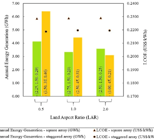
Land aspect ratio (LAR)
The optimal square array and staggered array layout configurations are simulated to achieve the lowest LCOE in each respective PV array layout as shown in Figure 4.7. This shows that the optimal square array and staggered array layout configurations are highly dependent on LAR. In addition, the simulated results have also shown that the staggered array layout configuration has a lower value of LCOE than that of the square array layout configuration for all the three cases considering LAR.
As a result, LAR is also one of the essential variables that can influence the optimal configuration of a solar power plant layout.
Conclusion
Future work
2015) "Modelling, analysis, and comparison of solar photovoltaic array configurations under partial shade conditions", Solar Energy. 2011) 'A review of photovoltaic leveled electricity costs', Renewable and Sustainable Energy Reviews, 15(9), pp. 2010) 'General Formula for On-Axis Sun-Tracking System', in Solar Collectors and Panels, Theory and Applications. 1991) "Central Station Solar Photovoltaic Systems: Field Layout, Tracker, and Array Geometry Sensitivity Studies", Solar Energy.
Elsevier Ltd (Woodhead Publishing Series in Energy), 2(3–4), p. 2013) “Sensitivity of kaleidoscope homogenizers to shading”, Solar Energy.