Drive Signal Simulation through Vehicle Suspension Modeling

THROUGH VEHICLE SUSPENSION MODELING

MOHAMMAD ARIF NURHADIYANTO

MECHANICAL ENGINEERING DEPARTMENT UNIVERSITI TEKNOLOGI PETRONAS

MAY 2005

I, MOHAMMAD ARIF NURHADIYANTO

hereby allow my thesis to be placed at the Information Resource Center (IRC) of Universiti Teknologi PETRONAS (UTP) with the following conditions:

1. The thesis becomes the property of UTP.

2. The IRC of UTP may make copies of the thesis for academic purposes only.

3. This thesis is classified as

Confidential

Non-confidential

Mohanimad Arif Nurhadiyanto

Sidoarum I, Flamboyan 3 Godean, Sleman

Yogyakarta 55564

Indonesia

Date: 19 July 2005

Endorsed by

•O.

Rashid Abdul Aziz

Mechanical Engineering Department Umversiti Teknologi Petronas 31750 Tronoh, Perak Darul Ridzuan Malaysia

Date: 19 July 2005

Approval by Supervisor

The undersigned certify that they have read, and recommend to The Postgraduate Studies Programme for acceptance, a thesis entitled "Drive Signal Simulation

through Vehicle Suspension Modeling" submitted by Mohammad Arif Nurhadiyanto for the fulfillment of the requirements for the degree of

Master of Science in Mechanical Engineering

Date: 19 July 2005

Lashid Abdul Aziz

W7 /W

11

Drive Signal Simulation through Vehicle Suspension Modeling By

Mohammad Arif Nurhadiyanto

A THESIS

SUBMITTED TO THE POSTGRADUATE STUDIES PROGRAMME

AS A REQUIREMENT FOR THE

DEGREE OF MASTER OF SCIENCE

IN MECHANICAL ENGINEERING

BANDAR SERIISKANDAR,

PERAK

JULY 2005

i n

citations which have been duly acknowledged. I also declare that it has not been previously or concurrently submitted for any other degree at UTP or other institutions.

Signature

Name Mohammad Arif Nurhadiyanto

Date 19 July 2005

IV

To my mother and father

who waited so long for this

I would like to gratefully acknowledge the enthusiastic supervision of Dr. Abdul Rashid Abdul Aziz during this work. I thank Pn Haslina and Rosle Yaakub for opening a golden opportunity to me. Staffs of the Proton Berhad are thanked for numerous stimulating discussions, help with experimental setup, and general advice; in particular I would like to acknowledge the help of Azmihan Arifin, Syammim, Wahab Lung, Zuliana Kamaruzaman, and Jayakanthan for their support. Dr. Ing. Yul Y. Nazaruddin, is thanked for his assistance with all types of technical problems.

I am grateful to all my friends from Umversiti Teknologi Petronas, for being the surrogate family during the many years I stayed there and for their continued moral support there after. From the staff, Pn. Norma, Ir. Idris, En. Azhar, En. Sani, Hazlin, Suhaily, Ustaz Cahyono, are especially thanked for their care and attention.

Finally, I am forever indebted to my parents and my family for their understanding, endless patience, and encouragement when it was most required. I am also grateful to Fadli and Arief for their support.

Arif

July 2005

VI

Road simulation testing of vehicles is often performed using a four posters road simulator. Four hydraulic actuators are used to replicate motions recorded during a previous test-drive using a drive signal. Typically, recordings are made of the vehicle sprung and unsprung accelerations at each of the four corners of the vehicle during an actual field-test. The hydraulic actuators are then driven and iterative tuning is performed such that the vehicle sprung and unsprung accelerations track those measured in the field.

Thus realistic suspension movements can be reproduced with the drive signal obtained from the iterative approach.

The overall goal of this research is to replace this iterative tuning which is specific for certain model of a car with a suspension system model. Acceleration data obtained from driving two test vehicles over selected well-defined sections of a test-track at constant speed were used for conducting this research. In modeling of the car suspension, the model of the system is assumed to be a quarter vehicle model and a rigid body system. Inputs to the system are the sprung and unsprung mass vertical accelerations. The output of the model is the drive signal estimation.

Two approaches of modeling have been applied for characterizing the dynamics of vehicle suspension. In the first approach, a linear model is derived from the equation of motion of vehicle suspension and a transfer function model is produced. In the second approach, a nonlinear modeling is used which treats the suspension as a black box model and considers only on the input and output of the suspension system.

Comparison of the results obtained from the two modeling approaches was then made and the errors were quantified. RMS error produced from the nonlinear modeling is found to be 2.4 % as compared to the linear modeling which produced a 14.5 % RMS error. This modeling result agreed with prior prediction that the simulated drive signal produced from the nonlinear modeling could better track the iterated drive signal rather than the linear modeling.

v n

Ujian simulasi jalan raya untuk kenderaan dilakukan dengan menggunakan "four posters road simulator". Empat pendorong hidrauhk digunakan untuk mengimbas pergerakan yang direkod semasa pandu uji dengan menggunakan signal pengendalian.

Kebiasaannya pecutan jisim terpegas dan jisim tak-terpegas pada empat penjuru kenderaan akan direkodkan semasa ujian praktikal dijalankan. Pendorong hidraulik akan digerakkan dan penalaan iteratif dijalankan sebagaimana pecutan jisim terpegas dan jisim tak-terpegas dianalisis semasa ujian praktikal. Oleh itu, pergerakan sebenar suspensi boleh dihasilkan daripada signal pengendali melalui penalaan iteratif yang telah dibuat.

Objektif kesuluruhan projek ini adalah untuk menggantikan penalaan iteratif yang yang khas untuk sebuah model kereta dengan model sistem suspensi. Analisis data pecutan yang diperolehi daripada ujian keatas kedua-dua jenis kereta pada halaju malar telah digunakan di dalam kajian ini. Kereta tersebut diuji pada jarak yang sama di atas sebuah litar. Suspensi ini hanya dimodelkan daripada suku bahagian kenderaan dan adalah sistem yang tegar. Nilai yang bertindak pada sistem adalah pecutan menegak daripada jisim terpegas dan jisim tak-terpegas. Hasil daripada model ini adalah anggaran signal pengendali.

Untuk memodelkan suspensi kendaraan, dua pendekatan telah digunakan untuk mengklasifikasikan pergerakan suspensi. Pendekatan pertama, persamaan pergerakan suspensi kenderaan melalui model linear dibuat dan perubahan fungsi model diperolehi.

Sementara itu, untuk pendekatan kedua, model tidak-linear dibina berdasarkan suspensi yang berfungsi sebagai model "kotak hitam". Hanya data yang dimasukkan dan dikeluarkan diambilkira untuk pendekatan kedua.

Kedua-dua keputusan daripada pendekatan diatas diperolehi dan dibandingkan.

Daripada keputusan tersebut, peratus ketidak tepatan telah dikira. Ketidak tepatan untuk RMS hasil daripada model tidak-linear adalah 2.4% dibandingkan dengan 14.5% apabila model linear digunakan. Keputusan daripada simulasi ini telah membuktikan bahawa model tidak-linear memberi keputusan yang lebih baik jika di bandingkan dengan model

linear.

v i n

Status of thesis i

Approval Page ii

Title Page hi

Declaration iv

Dedication v

Acknowledgement vi

Abstract vii

Abstrak viii

Table of Contents ix

List of Tables xii

List of Figures xiii

CHAPTER 1 : INTRODUCTION 1

1.1 Research Background 1

1.2 Research Objective 2

1.3 Research Scope 3

1.4 Research Methodology 3

1.5 Thesis Outline 7

CHAPTER 2 : LITERATURE REVIEW 8

2.1 Vehicle Suspension Modeling 8

2.2 Road Profiling 9

2.3 Nonlinear Modeling of Vehicle Suspension 10

2.4 Conclusion 10

CHAPTER 3 : MODELING OF VEHICLE SUSPENSION SYSTEM 12

3.1 Vehicle Suspension System 12

3.2 Mathematical Modeling of Vehicle Suspension Systems 16

i x

3.2.2 State Space Model and Transfer Function Model 17

3.3 Artificial Neural Network 18

3.4 Neural Network Modeling of Vehicle Suspension System 24

CHAPTER 4 : TESTING AND DATA ANALYSIS 29

4.1 Test Procedure 29

4.1.1 General Test Design 29

4.1.2 Test Preparation 33

4.1.3 Instrumented Ride Vibration Measurement 36

4.1.4 Test Rig Description 37

4.2 Data Processing 38

4.2.1 China Road Data 38

4.2.1.1 Signal Filtering 42

4.2.1.2 Signal Integration 45

4.2.1.3 Signal Differentiation 48

4.2.2 Proton Test Track Data 50

4.2.2.1 Signal Filtering 52

4.2.2.2 Signal Integration 55

4.2.2.3 Signal Differentiation 57

CHAPTER 5 : RESULTS 59

5.1 Mathematical Modeling Results 59

5.2 Artificial Neural Network Modeling Results 67

CHAPTER 6 : DISCUSSION 69

6.1 Linear Modeling 69

6.2 Artificial Neural Network Modeling 71

CHAPTER 7 : CONCLUSION 73

APPENDICES 78

XI

Table 4.1 Tire parameters of test vehicles 33

Table 4.2 Suspension parameters of Proton X 34

Table 4.3 Suspension parameters of Proton Y 35

Table 6.1 RMS error for China road drive signal modeling 70 Table 6.2 RMS error for Proton test-track drive signal modeling 70 Table 6.3 RMS error for China road drive signal modeling using ANN 72

x n

Figure 1.1 China road modeling steps 4

Figure 1.2 Proton test-track modeling steps 5

Figure 1.3 Artificial neural network modeling steps 6

Figure 3.1 SAE vehicle axis systems 13

Figure 3.2 Ride dynamic system 13

Figure 3.3 Quarter-car model 14

Figure 3.4 Tire spring rate 15

Figure 3.5 Characteristics of neuron 19

Figure 3.6 Common activation functions 20

Figure 3.7 A single layer neural net 21

Figure 3.8 A multilayer neural net 21

Figure 3.9 Backpropagation neural network with one hidden layer 22 Figure 3.10 Algorithm of backpropagation neural net 23-24 Figure 3.11 ANN model structure for vehicle suspension 28

Figure 4.1 Comparison between industrial practice and cunent approach 30

Figure 4.2 FRF calculation 32

Figure 4.3 Iterative process 32

Figure 4.4 Proton simulation test track 36

Figure 4.5 Sensor placement 37

Figure 4.6 Laboratory testing set up 38

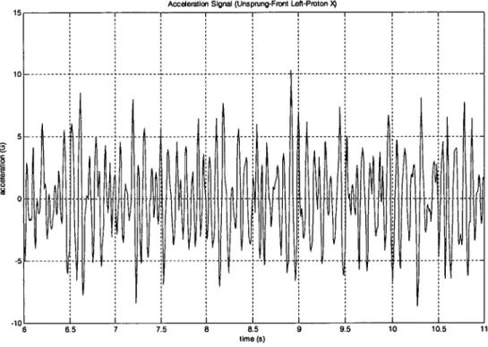
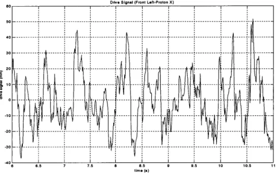
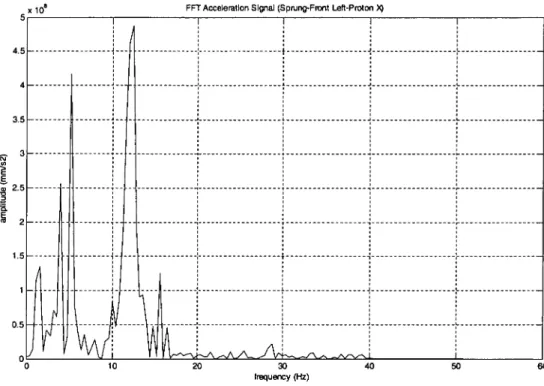
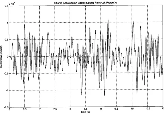
Figure 4.7 Acceleration signal (unsprung-front left-Proton X) 39 Figure 4.8 Acceleration signal (sprung-front left-Proton X) 39 Figure 4.9 Iterated drive signal (front left-Proton X) 40 Figure 4.10 FFT acceleration signal (unsprung-front left-Proton X) 40 Figure 4.11 FFT acceleration signal (sprung-front left-Proton X) 41 Figure 4.12 FFT iterated drive signal (front left-Proton X) 41

x i n

Figure 4.14 Filtered acceleration signal (sprung-front left-Proton X) 43 Figure 4.15 Filtered iterated drive signal (front left-Proton X) 43 Figure 4.16 FFT - Filtered acceleration signal (unsprung-front left-Proton X) 44 Figure 4.17 FFT - Filtered acceleration signal (sprung-front left-Proton X) 44 Figure 4.18 FFT - Filtered iterated drive signal (front left-Proton X) 45 Figure 4.19 Velocity signal (unsprung-front left-Proton X) 46 Figure 4.20 Detrend velocity signal to remove DC offset

(unsprung-front left-Proton X) 46

Figure 4.21 Detrend velocity signal to remove DC offset

(sprung-front left-Proton X) 47

Figure 4.22 Displacement signal (unsprung-front left-Proton X) 47 Figure 4.23 Displacement signal (sprung-front left-Proton X) 48 Figure 4.24 Acceleration data comparison (unsprung-front left-Proton X) 49 Figure 4.25 Acceleration data comparison (sprung-front left-Proton X) 49 Figure 4.26 Acceleration signal (unsprung-front left-Proton X) 50 Figure 4.27 Acceleration signal (sprung-front left-Proton X) 51 Figure 4.28 FFT acceleration signal (unsprung-front left-Proton X) 51 Figure 4.29 FFT acceleration signal (sprung-front left-Proton X) 52 Figure 4.30 Filtered acceleration signal (unsprung-front left-Proton X) 53 Figure 4.31 Filtered acceleration signal (sprung-front left-Proton X) 53 Figure 4.32 FFT - Filtered acceleration signal (unsprung-front left-Proton X) 54 Figure 4.33 FFT - Filtered acceleration signal (sprung-front left-Proton X) 54 Figure 4.34 Velocity signal (unsprung-front left-Proton X) 55 Figure 4.35 Velocity signal (sprung-front left-Proton X) 55 Figure 4.36 Displacement signal (unsprung-front left-Proton X) 55 Figure 4.37 Displacement signal (sprung-front left-Proton X) 57 Figure 4.38 Acceleration data comparison (unsprung-front left-Proton X) 57 Figure 4.39 Acceleration data comparison (sprung-front left-Proton X) 58

x i v

(front left-Proton X) 61 Figure 5.2 Comparison: simulated and iterated drive signal

(front right-Proton X) 61

Figure 5.3 Comparison: simulated and iterated drive signal

(rear left-Proton X) 62

Figure 5.4 Comparison: simulated and iterated drive signal

(rear right-Proton X) 62

Figure 5.5 Unfiltered simulated drive signal (front left-Proton X) 63 Figure 5.6 FFT - unfiltered simulated drive signal (front left-Proton X) 64 Figure 5.7 Filtered simulated drive signal (front left-Proton X) 65 Figure 5.8 FFT - filtered simulated drive signal (front left-Proton X) 65 Figure 5.9 Simulated drive signal comparison at front left

(Proton X - Proton Y) 66

Figure 5.10 Simulated drive signal comparison at rear left

(Proton X - Proton Y) 66

Figure 5.11 Validation result of ANN model 67

Figure 5.12 Simulation result of ANN model 68

Figure 7.1 Drive signal comparison (front left-Proton X) 74 Figure 7.2 Drive signal comparison (rear left-Proton X) 74

x v

INTRODUCTION

This chapter describes a general overview of this research. Background information related to the topic of vehicle suspension system and the objective of the research are introduced. The scope of the research and the research methodology are also presented here. Finally an outline of the thesis and a brief description on the contents of each chapter are also presented.

1.1 Research Background

Research in vehicle suspension system has been an on-going study for decades, ever since the invention of automobiles. Engineers and researchers have been trying to fully understand the dynamic behavior of vehicle suspension as it is subjected to different road conditions and different driving conditions, such as moderate daily driving and extreme emergency maneuvers. They want to apply this finding to improve issues such as ride comfort and safety factor, and develop innovative design that will improve vehicle operations. With the aid of fast computers to perform complicated design simulations and high speed electronics that can be used as controllers, new and innovative concepts have been tested and implemented into vehicles. This type of research is mainly conducted by automotive companies and academic institutions.

Automotive companies, together with academic institutions, are constantly improving on the chassis design and development by re-engineering the suspension systems with new technology. For example, the recent developments of vehicle suspension system show that a marriage of vehicle suspension dynamics and electronics can improve both ride comfort and safety factor. Examples of such systems are semi- active and fully-active suspension. It enables damping characteristics of the suspension system to be set by a feedback controller in real time, thus improving the ride quality of the vehicle on different types of road conditions.

perform a simple laboratory test on each axle of the vehicle, to measure its dynamic characteristics. This information is then used to generate a numerical model of the response of the whole vehicle to a typical road type input. More detail information about this technique will be explained in the following section.

1.2 Research Objective

Fatigue and vibration testing of vehicles are often performed using a four posters road simulator, where the test vehicle sits on four hydraulic actuators which are used to replicate motions recorded during a previous road test. Typically, recordings are made of the body and chassis accelerations at each of the four corners of the vehicle. The hydraulic actuators are then driven with appropriate input signals so-called drive signal such that the body and chassis accelerations follow those measured in the field. Thus realistic suspension movements can be reproduced and the drive signal is obtained.

The cunent solution to this 'mission reproduction' involves an iterative, off-line procedure (Westwick et al., 1999). First, an identification experiment is performed by exciting the system with a relatively broad-band noise input. A linear Frequency Response Function (FRF) is estimated from the test data. The target outputs are then filtered using the inverse of the FRF, producing an initial input sequence. If, as is often the case, the initial input sequence does not cause the system to track the target outputs adequately, the inputs are refined. The inverse FRF is applied to track the error, and the result is added to the test input. This off-line refinement process iterates until sufficient tracking accuracy is obtained.

The overall goal of this research is to replace this iterative tuning which is specific for certain model of car with a deterministic method. Transfer function and state space model will be derived from vehicle suspension system to recreate the movement of suspension. It is then compared with nonlinear modeling results using Artificial Neural Network. It should be pointed out that the result of the modeling is not the road profile.

This research is trying to find the drive signal that accurately reproduces response the same as road simulator excitation using unsprung and sprung acceleration data.

Two models of Proton passenger cars with conventional suspension system were used for

this research. Two kinds of input (random and deterministic) were excited on each of the vehicle wheel. The acceleration sensors were mounted on the sprung and unsprung mass of the vehicle to measure its vertical acceleration. The lateral and longitudinal forces to the vehicle are assumed to be negligible. Two modeling approaches, i.e. mathematical and artificial neural network modeling, were used to model the system to get the drive signal. This simulated drive signal was then compared with the iterated drive signal which was reproduced from the road simulator.

Some assumptions are made in modeling the vehicle suspension system. The major assumptions for this research are:

1. The vehicle body is considered as a rigid body. Therefore in deriving the vehicle equation of motion, the vehicle body is treated as a rigid body system.

2. The system is viewed as a quarter car system.

3. The car parameters used in modeling the system are obtained from a certain car model. The car model used in this work cannot be revealed due to confidentially agreement with Proton

1.4 Research Methodology

This research attempted to compare transfer function (linear) model against neural network (nonlinear) model. The following steps describe the above two approaches:

1. Transfer function model.

Figure 1.1 shows the transfer function model approach using Proton X car model with

random signal input (China public road). Acceleration data was measured at sprung and

unsprung mass of the car at front left, front right, rear left, and rear right position. Iterated

drive signal was determined by 'mission reproduction' using road measured data (acceleration data) and road simulator.

i

filtering (low pass filter) (sprung, unsprung, drive signal)

X

integration (cumulative trapezoid)

to find v and x

(sprung, unsprung) X

check the reliability of integration process by applying

double differentiation to the results

(sprung, unsprung) X

mathematical modeling

description of the system X

free body diagram X

equation of motion I

state space model & transfer function model X

modeling results (simulated drive signal)

X

compare the drive signal between

iterative results (road simulator) and modeling results for all wheels (come out with RMS error)

Figure 1.1 China road modelingsteps.

Figure 1.2 uses two car models, i.e. Proton X and Proton Y, using Proton test- track as determimstic signal input. Acceleration data was measured at sprung and unsprung mass of the car at front left and rear left positions. Drive signal was not provided.

(sprung, unsprung) I

filtering (low pass filter) (sprung, unsprung)

X

integration (cumulative trapezoid)

to find v and x

(sprung, unsprung)

check the reliability of integration process by applying

double differentiation to the results

(sprung, unsprung) X

mathematical modeling description of the system

X

free body diagram X

equation of motion

state space model & transfer function model X

modeling results

filtering (high pass filter)

modeling results - final (simulated drive signal)

compare the simulated drive signal between

Proton X and Proton Y for front left and rear left wheel position (come out with RMS error)

Figure 1.2 Proton test-track modeling steps.

In the ANN modeling, the Proton test-track data was used for training process, whilst the China road data was used for simulation. Figure 1.3 shows the steps of the ANN modeling using Proton X car model.

select model structure

find the polynomial coefficients of the

system using discretization of the system equation of

motion and backward formulation

identification

(model iteration and estimation)

come out with appropriate network parameters and weight

validate model

simulate model

compare the drive signal between

iterative results (road simulator) and modeling results for front left and rear left position

(come out with RMS error)

Figure 1.3 Artificial neural network modelingsteps.

Comparison was then made between the transfer function model and neural network

model.

Chapter 1 describes general overview of this research. Background information related to the topic of vehicle suspension system and objective of this research are introduced. The scope of the research and the research methodology are also presented

here.

Chapter 2 briefly describes the published papers, journals, proceedings, that were found most relevant and complimentary to this research.

Chapter 3 explains the dynamic modeling of vehicle suspension system. The concept of vehicle suspension system and the derivation of linear and nonlinear modeling of vehicle suspension are presented in this chapter.

Test procedure and data analysis methodology for obtaining the best data are provided in chapter 4. There are two kinds of data that were obtained, i.e. road data from

China and track data from Proton test-track.

Chapter 5 describes the modeling results of vehicle suspension systems. In the first section of this chapter, the results of mathematical modeling for both China road and Proton test-track will be presented. It is then followed by nonlinear modeling results using artificial neural network.

Chapter 6 briefly discusses the main issue in this research. The results of vehicle suspension modeling for both linear and nonlinear modeling are the main topics briefed in this chapter.

Finally, the conclusion of the research is provided in chapter 7.

LITERATURE REVIEW

This chapter provides information on past research on vehicle suspension modeling to recreate the drive signal using analytic and nonlinear algorithms. An extensive literature search was conducted with the most relevant results presented in this chapter. Although the nonlinear modeling of vehicle suspension has been addressed in a number of articles, none of the previous studies tried to compare the modeling results between linear and nonlinear modeling with the same input-output. This research has also succeeded on producing the drive signal for both random and determimstic road profile input.

2.1 Vehicle Suspension Modeling

Modeling of vehicle suspension and its components have been studied for several decades. Vast assortments of models have been proposed and are used for many different circumstances. A study by Tao (2000), addressed a modeling suspension damper modules using LS-Dyna. It describes a finite element model of a suspension damper and accurately represents component interactions and force distributions within the module.

The study conducted by Ruihong and Runhua (1999), has successfully reduced the variation of velocity characteristic of the shock absorber in a car using modern robust optimal design method, applied to its structural parameter design. They tried to analyze the influences of the parameters on velocity characteristics and the robust values which can improve velocity characteristic. The study by Rao and Gruenberg (1997) described a new testing and analysis methodology for obtaining equivalent linear stiffness and damping of automotive shock absorbers for use in system-level chassis and vehicle computer aided engineering models for noise and vibration prediction.

A study by Lacombe (2000) addressed the tire model for simulations of vehicle motion on high and low friction road surfaces. He developed an on-road analytical tire model to predict tire forces and moments at the tire/road interface. Takahashi et al. (2000) presented a new tire model of the overturning moment (OTM) characteristics and the

term of the residual pneumatic scrub. The concept of the new model is to identify the difference between the simple model and the measurements to the newly defined functions. They investigated the influence of tire OTM on the vehicle rollover. The study conducted by Hankook Tire Co., Ltd. (2001) describes the role of tire modeling on the design process of a tire and vehicle system.

Renner (2000) proposed an Empirical Dynamic Models (EDM) for nonlinear suspension components. The models addressed in this study are faster to be created rather than analytical models, more accurate than other black box methods, and faster model execution. Automotive testing company, MTS, has proposed EDM to accelerate new suspension development. ElBeheiry and Kamopp (1996) investigated five types of suspensions: fully active, the limited active, the optimal passive, the actively damped, and the variable damper systems. Comparisons were made among these systems in terms of RMS response, frequency domain predictions, and eigen-frequency behavior as functions of disturbance intensity. They tried to optimize the variable parameter suspension to use the available suspension deflection to provide maximum isolation.

2.2 Road Profiling

The measurement method of road profile have been studied and conducted a great deal by many researchers and companies. Sayers and Karamihas (1998) released the Little Book of Profiling, the most popular reference related with this area of research. It gives a basic information about measuring and interpreting road profiles. The study conducted by Katech (2000) describes the construction of Dynamic Road Profiling Devices (DRPD) and the signal processing for advanced double integration and road profiling for AEIPR (an Accelerometer Established Inertial Profiling Reference) method.

Some studies related with the process of simulation 'from the field to the laboratory' have also been conducted by many researchers. Westwick et al. (1999) models the dynamic of a car attached to a vibration test rig and presented a realistic simulation of a nonlinear automobile suspension. The overall goal of their research is to replace the mission reproduction which is involves an iterative, off-line procedure with an online controller. Storer et al. (1998) characterized the transfer of road surface excited

vibrations through vehicle suspension system. They applied a technique called Transfer Path Analysis, originally developed to study the aspect of powertrain-induced vibrations of the vehicle body, to the suspensions of the complete vehicle being tested on the road or in the laboratory on a road simulator.

2.3 Nonlinear Modeling of Vehicle Suspension

The nonlinear modeling of vehicle suspension has been such an important issue in the automotive research activities that many studies have addressed different aspects and method of these modeling. Felicia and loan (2000) applied neural networks to vehicle suspension system. They focused on exploring the possibility of deriving the (semi)active suspension system controllers based on the artificial intelligence strategy, and verifying the proposed procedure of derivation by simulation results. Lin and Kanellakopoulos (1995) proposed a nonlinear backstepping design for active suspension system which aims to improve the trade-off between ride quality and suspension travel. They showed that the intentional introduction of nonlinearity through the controller into an otherwise linear system can be beneficial in cases where the desired closed-loop response is different operating regions. Yul and Yamakita (1999) presented an alternative approach to identify suspension system model using neuro-fuzzy technique. By using this approach, the nonlinear characteristics of the suspension system have accommodated.

Westwick et al. (1999) addressed a nonlinear identification of automobile vibration dynamic. They developed a technique for identifying a restricted class of nonlinear state space systems, a structure which can be used to model a wide variety of systems.

2.4 Conclusion

The nonlinear modeling of vehicle suspension to recreate the drive signal is of great importance to the automotive industry and has therefore been the subject of many studies.

Previous studies have addressed many aspects and methods of the modeling and have attempted to develop models based on the actual measurement from a running test vehicle. Modeling of suspension component, such as shock absorber, and tire modeling, especially in dynamic condition, has also been studied a great deal by many researchers.

With the aim of improving the ride comfort behavior of vehicles for road-surface

excitation, a great deal of researchers and companies have been trying to understand in detail the dynamic characteristics of the suspension systems and the transfer of vibration through the vehicle suspension.

Most of the previous studies have been limited in the modeling technique and experimental data for verification. The previous research applied only one type of modeling and one type of input. This research tried to compare the modeling results between linear and nonlinear modeling with the same input-output. This research has also attempted to reproduce the vehicle suspension movement by determining the drive signal for both random and deterministic road profile input.

CHAPTER 3

MODELING OF VEHICLE SUSPENSION SYSTEM

This chapter briefly describes the dynamic modeling of vehicle suspension system. The concept of vehicle suspension system, includes a quarter-car system is first presented in this chapter. It then describes the derivation of linear and nonlinear modeling approaches for identifying the characteristic of vehicle suspension.

3.1 Vehicle Suspension System

The excitation source (i.e. vertical forces exerted by the road on a tire) is transmitted to the vehicle body through the vehicle suspension system. This system allows its components to absorb the energy of the road roughness so passengers can have a smooth ride. In other words, it provides vertical compliance so the wheels can follow the uneven road, isolating the body from roughness in the road. The others primary functions of a suspension system are to (Gillespie, 1992):

• Maintain the wheels in the proper steer and camber attitudes to the road surface.

• Resist roll of the chassis.

• React to the control forces produced by the tires - longitudinal (acceleration and braking) forces, lateral (cornering) forces, braking and driving torques.

• Keep the tires in contact with the road with minimal load variation.

To study the fundamental behavior and characteristics of vehicle suspension system, it is necessary to understand the basic concepts of vehicle dynamics, ride, and quarter car model. This section presents the necessary information on those subjects. The vibration-absorber-components of vehicle are also described in this section.

Vehicle Dynamics

The subject of 'vehicle dynamics' is concerned with the movements of vehicles on a road surface. The forces imposed on the vehicle from the tires, gravity, and aerodynamics determine dynamic behavior of the vehicle. The vehicle and its

components are studied to determine what forces will be produced by each of these sources at a particular maneuver and trim condition, and how the vehicle will respond to these forces. Understanding vehicle dynamics can be accomplished at two levels-the empirical and the analytical. The empirical understanding derives from trial and ereor from which one learns about the factors that influence the vehicle performance. The empirical method, however, can often lead to failure. Without a mechanistic understanding of how changes in vehicle design or properties affect performance, extrapolating past experience to new conditions may involve unknown factors which may produce a new result, defying the prevailing rules of thumb. For this reason, engineers favor the analytical approach. The analytical approach attempts to describe the mechanics of interest based on the known laws of physics so that an analytical model can be established and represented by differential equations that relate forces or motions of interest to control inputs and vehicle or tire properties.

Ride

Vehicles travel at high speed, and as a consequence experience a broad spectrum of vibrations. These are transmitted to the passengers either by tactile, visual, or aural paths.

The term 'ride' is commonly used in reference to tactile and visual vibrations, while the aural vibrations are categorized as noise. Alternatively, the spectrum of vibrations may be divided up according to frequency and classified as ride i.e. 0-25 Hz, and noise i.e. 25- 20000 Hz (Gillespie, 1992). The lower-frequency ride vibrations are manifestations of dynamic behavior common to all rubber-tired motor vehicles. Thus, the study of these modes is an important area of vehicle dynamics. As an aid in developing a systematic picture of ride behavior, it is helpful to think of the overall dynamic system as shown in Figure 3.2.

Excitation Sources

Road Roughness

Tire/wheel Driveline

Engine

y Vehicle Dynamic

Response

Vibration

^ >

Ride

Perception

Figure 3.2 Ride dynamic system.

(adoptedfrom: Gillespie, Fundamentals of Vehicle Dynamics, 1992/

Quarter-car Model

At the most basic level, all vehicles share the 'ride isolation' properties common to a sprung mass supported by primary suspension systems at each wheel. The dynamic behavior of this system is the first level of isolation from the roughness of the road. The essential dynamics of the vehicle suspension system can be simplified and represented by a quarter-car model as shown in Figure 3.3.

1

^xb

ix, J,

Figure 3.3 Quarter-car model.

It consists of a sprung mass (nib) supported on a primary suspension, which in turn is connected to the unsprung mass (mt). The suspension has stiffness (ks, kp) and damping (cs) properties. Tire, which interacts between the road and the car, has a spring rate (kt) to cushion the car against road inegularities.

A quarter-car model is the simplest model that includes a proper representation of the problem of controlling wheel load variation. It contains no representation of geometric effects of having four wheels or the use of front suspension state information to improve the performance at the rear. However, it does appear to contain the most basic features of the real problem and gives rise to design thinking. Thus, to demonstrate the application of identification algorithm on a manageable, nonetheless realistic, this research uses a continuous-time simulation of a quarter-car model.

The Tire

Motion of the vehicle is controlled almost entirely through the forces exerted on the tire by the road. The tire characteristics therefore have a major effect on handling problems.

The tire serves essentially three basic functions (Gillespie, 1992):

• It supports the vertical load, while cushioning against road ^regularity

• It develops longitudinal forces for acceleration and braking

• It develops lateral forces for cornering

The tire can be simply represented as a simple spring (kt), although a damper is often included to represent the small amount of damping inherent to the visco-elastic nature of the tire. The tire spring rate can be illustrated as Figure 3.4.

Figure 3.4 Tire spring rate.

Spring

Spring can be defined as a component that is designed to have a relatively low stiffness compared with normal rigid members, thus making it possible to exert a force that varies in a controlled way with the length of the member. Springs are generally classified according to the material used and the way that the forces and corresponding stresses occur. In a quarter-car model, spring is represented as ks.

Damper

It is one of the most important parts on vehicle suspension. The damper is commonly known as the shock absorber, although the implication that shocks are absorbed is misleading. Contrary to their name, they do not absorb the shock from road bumps.

Rather the suspension absorbs the shock and the shock absorber's function then is to dissipate the energy put into the system by the bump (Dixon, 1996). The primary purposes of a damper are (Dixon, 1996):

• To dissipate any energy in the vertical motion of body or wheels.

• To optimize vehicle control behavior by preventing response overshoots.

• To minimize the influence of unavoidable resonance.

In a quarter-car model, damper is represented as cs.

Parasitic Coefficient

Apart from the deliberately introduced suspension spring and tire spring rate, there are other sources of springing material inherent in the system. One is rubber bushes. In a quarter-car model, parasitic coefficient is represented as kp.

Mass

The total mass of the vehicle may be considered to be divided into sprung mass (nib) and unsprung mass (mt). These terms refer to the component motion relative to the road.

Basically the sprung mass is the body and the unsprung mass is mass of the wheels and axles. The term "wheel" may be used in a wide sense to include the whole of the rotating element including the tire, or in a narrow sense to mean the part that connects the tire to

the hub.

3.2 Mathematical Modeling of Vehicle Suspension System

3.2.1 Description of the System

As previously mentioned, the essential dynamics of vehicles can be expressed by a two- mass model as shown in Figure 3.3. It contains two vertical degrees of freedom: the displacement of the unsprung mass, xt , and displacement of the sprung mass, Xb. The road displacement input is denoted by xr. Ks, kp, and kt are the spring coefficient of suspension, parasitic, and tyre, respectively, and cs is the damper coefficient.

By applying Newton's second law of motion to the quarter-car system as showed in Figure 3.3, the equation of motion of the system can be written as

.. cs . cs . , (kp+ks+kt) (kp+ks) kt

x,+—xt—-**+ — xt p- *6=—*r (3.1)

mt m, mt mt mt

c. . c. . (*„+*,) & +k,)

— Xt H —

xb-^xt+^xb-^ s-x,+^ s-xb=0

(3.2)

3.2.2 State Space Model and Transfer Function Model

• State Space Model

Following Ihsan (2002), by using the state variables:

x\ xi x2 — xb x3 — xt

xA — xb

Eq. (3.1) and (3.2) can be rewritten as

0 0 1 0

*1 x2

0

(kp+ks+kt)

0 0 1

2*_

x3 -X4.

m,

(kp+ks)

m,

(kp+ks)

mt

£s_

m,

c

mk mu m,. mk

— — 0

xx 0 x2

+ K

x3

m,

Xa

0

Equation (3.3) is the state space model representation of vehicle suspension system.

Transfer Function Model

(3.3)

Another way of representing the mathematical model of vehicle suspension system is the transfer function model of its system. The model can be obtained by applying Laplace transform and Cramer law to Eq. (3.1) and (3.2).

First, Eq. (3.1) and (3.2) can be written in a matrix form,

~mt

0" x\

+

0

mb\lxb\

^{c. +}

The Laplace transform of Eq. (3.4) is

nls2+css +kp+ks+kl -(css +ks+kp) -(css +k5+kp) mbs2+css +kp+ks

Xt(s) LXb(s\

k,Xr(sj

0

ktxr

0

(3.4)

Next, using Cramer law,

mts2 + css + k + ks + kt ktXr(s) Xh(s) =

-(css + ks +kp) ⁰

m.s + cs + kn + k, + k, - (c,s + k + kn)

Xb{s) =

TF(s) =

(css + ks +kp)

(c,s + k,+k)ktXr(s)

mhs_o + c,s + kn + k,_{s p s}

(mts2 + css + k +k,+ kt)(mbs2 + c,s + k + ks) - (css + k + ks)2

Xr (s) (m,52 + css + k +k,+k, ){mbs2 +css + k +ks)- (css + k + ks f

(css + ks+kp)k,

k,Xr(s) -(css + ks+kp) Xb{s) = - 0 mhs2 + c,s + kn+k,o s p s

m.s2+c,s+ kn+k+k._{t s p s t} -(c,s + k+k„)_{v s s p y}

~{c

ss +ks+kp) mbs2+css +

-kn+k,

p '

Xt(s) =

(mbs2 +css + ks+kp)klXr(s)

(m.s2 +css +kp+ks +kl)(mbs2 +css +kp +ks)-(css + kp +ks)2

TF(s) =

Xr(s) (m,s2 +css+ kp +ks +kt)(mbs2 +css + kp +ks)-(css + kp +ksf (mbs2 +css + ks+k )k,

(3.5)

(3.6)

Eq. (3.5) is the sprung mass-road transfer function model, while Eq. (3.6) is the unsprung

mass-road transfer function model.

3.3 Artificial Neural Network

Artificial Neural Network (ANN) is one of nonlinear modeling method of dynamics systems. It has capability to control a system with uncertainty relationships between input and output. It works as biological neural networks therefore ANN has an ability to imitate the function and characteristics of human neural networks. In other words, the main strength of ANN is its ability for learning and training, as human characteristics.

It is obvious that vehicle suspension components, such as damper, bushing, even spring has a nonlinear characteristic. Due to this nonlinearity, ANN with its nonlinear characteristic capability, was applied to model the vehicle suspension system.

Architectures/Structures ofNeural Network

Artificial neural networks have been developed as generalizations of mathematical models of human cognition or neural biology, based on the assumptions that (Fausett,

1994):

• Information processing occurs at many simple elements called neurons.

• Signals are passed between neurons over connection links.

• Each connection link has an associated weight, which, in a typical neural net, multiplies the signal transmitted.

• Each neuron applies an activation function (usually nonlinear) to its net input (sum of weighted input signals) to determine its output signal.

A neural network is characterized by (1) its pattern of connection between the neutrons (called its architecture), (2) its method of determining the weights on the connections (called its training, or learning, algorithm), and (3) its activation function.

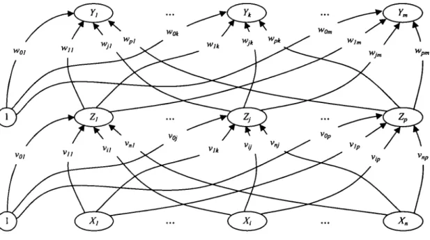
Figure 3.5 shows a simple processing element called neuron, unit, cell, or node. A neuron can send only one signal at a time, although that signal is broadcast to several other neurons. It is illustrated in Figure 3.5 that the neuron has input vector x = (xi, ... , Xj, ... ,xn).

y_inj !

i yj

Figure 3.5 Characteristics ofneuron.

Each neuron is connected to other neurons by means of directed communication links, each with an associated weight. The weights represent information being used by

the net to solve the problem. A bias can be included by adding a component x0 = 1 to the vector x, i.e., x = (1, xi, ... , Xj,... , xn). The bias is treated exactly like any other weight, i.e., woj = bj .

Each neuron has an internal state, called its activation or activity level, which is a function of the inputs it has received. Typically, a neuron sends its activation as a signal to several other neurons. As we can see from Fig 3.5, the output of the neuron is yj.

i t

y_inj = Yuxiwa

i=0

n

=woj+£x,.w..

1=1

:vZ*.-w*

1=1

yJ = f(y_inj)

As mentioned before, the basic operation of an artificial neuron involves summing its weighted input signal and applying an output, or activation function. There are several functions that can be used for activation function as illustrated in Figure 3.6.

f(x)

Identity Function Binary Step Function Hyperbolic Tangent Function

Figure 3.6 Common activationfunctions.

(adoptedfrom: Hines, Fuzzy and Neural Approaches in Engineering, 1994).

From those three functions, hyperbolic tangent function is the most widely used in application from these following reasons:

• Nonlinear characteristics

• Continuous function

• Simple relationship between the value of the function at a point and the value of the derivative at that point (reduces the computational burden during training).

The hyperbolic tangent is

= exp(x) - exp(-x)

exp(^) + exp(-x) The derivative of the hyperbolic tangent is

h'(x) = \l +h(x)ll-h(xj\

The arrangement of neurons into layers and the connection patterns within and between layers is called the net architecture. The net illustrated in Figure 3.7 consist of input units and output units.

CX>

CE>

CED

Fig 3.7 A single layer neural net.

Neural nets are often classified as single layer or multilayer. In determining the number of layers, the input units are not counted as a layer, because they perform no computation. The net illustrated in Figure 3.7 is single layer net, while the net shown in Figure 3.8 has two layers, consist of input units, output units, and one hidden unit.

w2

Fig 3.8 A multilayer neural net.

Backpropagation Neural Net

A multilayer neural network with one layer of hidden units (the Z units) is shown in Figure 3.9. The output units (the Y units) and the hidden units also may have biases. The bias on a typical output unit Yk is denoted by w0k ; the bias on a typical output unit Zj is denoted by v0j. Only the direction of information flow for the feedforward phase of operation is shown. During the backpropagation phase of learning, signals are sent in the

reverse direction.

Fig 3.9 Backpropagation neural network with one hidden layer.

(adoptedfrom: Fausett, Fundamentals ofNeural Networks, 1994).

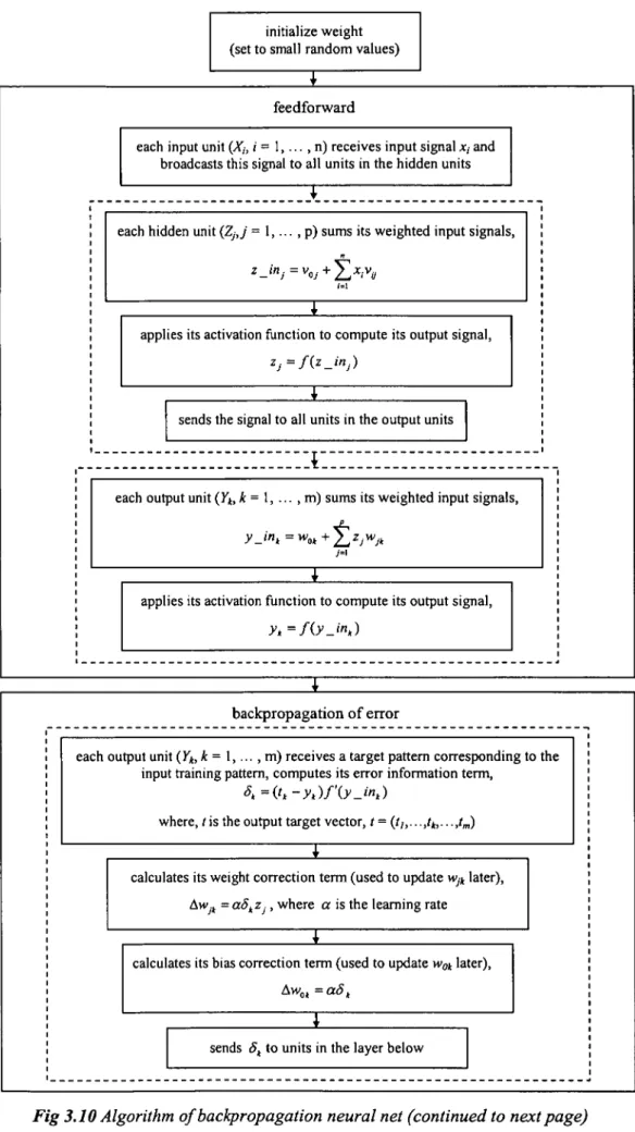
The training of a network by backpropagation involves three stages: the feedforward of the input training pattern, the calculation and backpropagation of the associated ercor, and the adjustment of the weights. The algorithm of backpropagation neural net is illustrated in Figure 3.10

initialize weight (set to small random values)

X

feedforward

each input unit (Xit i = 1, ... , n) receives input signal xt and broadcasts this signal to all units in the hidden units

T

each hidden unit (ZjJ = 1,... , p) sums its weighted input signals,

n

X

applies its activation function to compute its output signal,

^j =/(z_'";) X

sends the signal to all units in the output units

:::x::::::::::::::::::;:::::__

each output unit (Yh k = 1, ... , m) sums its weighted input signals,

•Jv

y-i

X

applies its activation function to compute its output signal, yt=fiyjnk)

X

backpropagation of error

each output unit (Yk,k= 1, ... , m) receives a target pattern corresponding to the input training pattern, computes its error information term,

St=(.tk-yk)fXy_ink)

where, t is the output target vector, / = ('/,•••,'*,•••,'«) X

calculates its weight correction term (used to update wJk later), Awjk = a5kZj, where a is the learning rate

T

calculates its bias correction term (used to update wok later), Aw0k = aSk

X

sends Sk to units in the layer below

Fig 3.10 Algorithm ofbackpropagation neural net (continued to nextpage)

A

each hidden unit (Zj,j = 1,..., p) sums its delta inputs (from units in the layer above),

m

5J"j =ZJ*wy*

X

multiplies by the derivative of its activation function to calculate its error information term,

SJ = S_inJf'{z_inJ)

X

calculatesits weight correction term (used to update Vy later), Av,j = aSjX,

X

calculatesits bias correction term (used to update v0y- later), Av0J = aSj

update weights and biases

each output unit (Yk, k = l,...,m) updates its bias and weights (j = 0,...,p):

wJk {new) = wJk (old)+ AwJk

I

each hidden unit (Zj,j = 1,...,p) updates its bias and weights (/ = 0,.. .,n):

v..(new) = wff(oW) + Avj/.

Fig 3.10 Algorithm ofbackpropagation neural net.

3.4 Neural Network Modeling of Vehicle Suspension System

Determination ofModel Structure

The structure of ANN model is constructed by its composed parameters. Those parameters are number of layers, number of nodes in input, hidden, and output layer, activation function for each node in hidden layer and output layer, and the weights. The weakness of this modeling is no definite method to establish the network parameters.

Therefore, the only way to define the variables for getting the best model structure is iteration. Iteration can be performed by varying the network parameters.

One of the network variables, that is the number of layers, can be first determined.

Santosa (1998) stated that performance of network with one hidden layer compared with two hidden layers is not different for simple model such as quarter-car system. Therefore, two network layers were applied for constructing the model, consist of input layer, output layer, and one hidden layer.

The number of nodes in input layer can be determined by deriving the sprung and unsprung transfer function model to find its polynomial coefficient. Structure of ANN input layer can be written as

[ y(t-l) ... y(t-na) u(t-nk) ... u(t-nb-nk+l)]T (3.7)

where,

u = input signal y = output signal

na = number of past outputs used for determining the prediction nb = number of past inputs used for determining the prediction nk = time delay (usually 1)

then, by using coefficients na, nb, and nk, the number of input layer nodes can be

determined.

Firstly, the vehicle suspension transfer function is rewritten,

TF(s) =

Xb(s) _ (css + k5+kp)kt

TF(s) =

Xr (s) (mts2 +css +kp+ks+k, )(mbs2 +css +kp+ks)- (css +kp+ks )2

Xt(s) = (mbs2+bss +ks+kp)k,

Xr (s) (m,s2 +css +kp+ks+kt )(mbs2 +css +kp+ks)-(css +kp+ks f

By defining constants

<h-*-

^{a2 —}

^*,+*,

mb mt

mt aA ⁼

K+kP

m,

a>l = — (co0 is the natural frequency of the unsprung subsystem)

k mt

then from Eq. (3.5) and (3.6) the following equation is obtained

TF(~\-Xb(s) - a?02(a,j +a2; , „

lt \s) ~ „ , x - —r—,—:—ns—:

Xb{s) = a>20(a,s +a2)

:—jtt- r - t (3.8)

Xr(s) s4 +(a, +a3)s3 +(a2 + a4 +col)s2 +a^s +a2(o\

Xt(s) _ a>l(s2 +ais +a2)

Xr(s) s4 +(a, +a3)s3 +(a2 +a4 +a>l)s2 + a^s + a2co\

ms) =^-= 4., , 3 T . ' T'',. — r (3-9)

By letting Xb,Xt as input and Xr as output variable, Eq. (3.8) and (3.9) can be rewritten

Xb+{ax + a3)Xb +(a2 +a4 +co2)Xb+alo)2Xb + a2co2Xb =co2(aiXr+a2Xr) (3.10)

Xt + (al + a3)Xt + {a2 + a4 + co2)Xl +alco2Xl +a2a>lXt =a>l(Xr +axXr +a2Xr) (3.11)

n n n

By defining Xb =y(t-n), X, =z(t-n), an&Xr =u(t-ri), Eq. (3.10) and (3.11) can be written in discrete time equation,

y(t-4) + (al+a3)y(t-3) + (a2+a4+Q)2)y(t-2) + aico2y(t-l) + a2co20y(t)

.2../.. 1\ , _ ,.2

= axcoQu(t -1) + a2co0u(t)

z(r-4) + (<3, +a3)z(t-3) + (a2 + a4 + a>l)z(t -2) + axa>\z{f -1) + a2a>2Qz(t)

= co20u(t - 2) + axcolu{t -1) + a2colu(t)

By defining constants

_ a.col _(a2+a4+a>20) _(a,+a3) 1

A\~ 2 ' A1 ~ 2 ' 3 _ 2 ' ^4 - 2

Ct2G)Q ^2^0 fl2<y0 a2<2,0

D fl1^0 n ®0

B\ =1 V2 > #2 =' 2 2

a2a>0 a2<uo

(3.12)

(3.13)

then Eq. (3.12) and (3.13) can be written in basic equation as follows y(t) + A,y(t -1) + A2y(t - 2) + A3y(t - 3) + ^4 v(f - 4) = «(r) + 5lM(f -1)

v(0 + 4j/(* -1) + A2y(t- 2) + ^3 v(/ - 3) + A4y(t - 4) = m(0 + 5,u(f -1) + B2u(t - 2)

Consider y(t- na) = q'"ay(t) and u(t-nb) = q~nbu(t), then constants A and B can be expressed in time delay operator q~l with

A(q) - 1+ axq~l +a2q~2 + a3q'3 + a4q~*

B(q) = blq-1

for sprung mass, and

A(q) = 1+ axq'x + a2q 2+ a3q 3+a4q~

B(q) = bxq~l +b2q-2

for unsprung mass

Therefore, the polynomial coefficients of the models canbe determined.

For unsprung mass:

na = 4 nb = 3 nk=l

For sprung mass:

na = 4 nb = 2 n k = l

Using Eq. (3.7), the structure of input layer is

[ y(t-1) ... y(t-4) u(t-1)... u(t-3)]T for unsprung mass [ y(t-1) ... y(t-4) u(t-1)... u(t-2)]T for sprung mass

The number of node in hidden layer along with its activation function can only be determined by iteration since there is no certain method for it. Whilst, for determining the output layernodes, it is complied with the problem faced.

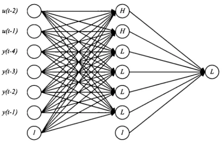
Iteration was performed using Matlab™ Neural Network Toolbox. The network

structure which produces the best model is illustrated in Figure 3.11.

input layer hidden layer output layer

Figure 3.11 ANN model structurefor vehicle suspension.

It is shown in Figure 3.11 that iteration was performed using input and output data at (t-2) and (t-1). (t-2) means that two past values were used for determining the renewed value. Each data was then forward-propagated to each hidden layer nodes which has activation function [ L L L L H H ]. L stands for linear activation function, while H stands for hyperbolic tangent activation function. Output from hidden layer was forward- propagated again to output layer with activation function [ L ]. Output from output layer node was then back-propagated to renew the weights. The weight is always corrected until satisfactory modeling is obtained.

CHAPTER 4

TESTING AND DATA ANALYSIS

The roughness in a road is the deviation in elevation seen by a vehicle as it moves along

the road. The roughness acts as a vertical displacement input to the wheels, thus exciting

ride vibrations. Yet the most common and meaningful measure of ride vibration is the acceleration produced. Therefore, for the purpose of understanding the dynamics of ride, the roughness should be viewed as acceleration input at the wheels.

This chapter explains the testing of Proton's suspension system to measure its ride dynamic characteristic for further modeling analysis. The test procedure encompasses

general test design, test preparation, instrumented ride vibration measurement, and test rig description. This chapter also describes the 'initial treatment' to the acceleration data

obtained, i.e. filtering and numerical integration for mathematical modeling purpose.

4.1 Test Procedure

4.1.1 General Test Design

A typical ride test consists of running vehicle over selected well-defined sections of road at constant speed and certain type of road was performed. Accelerometers were mounted

on the vehicle sprung and unsprung mass to measure its vertical acceleration. The field measured data was then brought to the laboratory for 'mission reproduction' using Remote Parameter Control (RPC) technique which is a built-in iteration software in the road simulator. Using the same car model, the actuators of the servo hydraulic four

posters road simulator were then driven and iterative tuning were performed such that the sprung and unsprung acceleration match those measured in the field. This iteration process involves estimation of a linearFRF (Frequency Response Function) from the test

data and refinement of the input sequence by using inverse of the FRF. Thus, realistic body motion and drive signal from the road simulator can be reproduced under controlled environment. A more detail explanation about this iteration technique will be described in

the next section.

As previously mentioned, the overall goal of this research is to replace this iterative tuning which is specific for certain model of car with a car suspension system

model. Once the model of the suspension has been determined, the drive signal can be recreated using acceleration data from the accelerometers and the car physical data. The

comparison between industrial practice procedure and modeling approach is illustrated in

Figure 4.1.

Record road or service data

transfer, analyze, edit data

}-

f > Ethernet •

Measure system FRF

System FRF

Estimate drive signal

Desireddata x [FRF]"' x Gain = Initial DriveEstimate

0 < Gain < 1

Calculate error and iterate

Corrected drive estimate

(iterated drive signal)

record road data

(sprung ft unsprung acceleration)

•

transfer, analyze, and edit data

1

••jjjj^^^H ^^^^•H^^^^l ••••MM •

modeling

^B

^•1 ••HIMBIi HB^{^^H}

transfer function of vehicle suspension

••I^^^K ••••••

1

simulated drive signal

II

• ^{^^^•••^H} W •

Figure 4.1 Comparison between industrialpractice and current modeling approach, (adoptedfrom: Arifin et al, Using Model Parameter toMonitor Vehicle Changes duringa Durability Test, 2000)

Remote Parameter Control

Remote Parameter Control (RPC) is an advanced simulation technique that is used to replicate and analyze 'in service' vibrations and motions of a specimen using a dynamic mechanical system in a controlled laboratory environment. RPC was developed by MTS Systems Corporation which is then applied to their product, i.e. road simulator.

Refer to Figure 4.1, the RPC process can be explained as follows (Arifin et al.,

2000):

1. Vehicle instrumentation and data collection.

• The test vehicle is instrumented with accelerometers and data recorder.

2. Edit and reduce data.

• The measured data is converted to RPC file format and analyzed using the RPC III TEDIT program.

• Data is reduced to the required data length.

• The acceleration data is run through the RPC HI 'remove_trend' program.

This program removes the slope in the data. The slope of the data is removed to remove any drift in the accelerometers during data collection.

• A filter is constructed with a band-pass frequency of 0.6-50 Hz (typical for a servo-hydraulic four posters). The filter is applied to each of the time

histories.

3. Measure system FRF (Frequency Response Function).

• The purpose of measuring the FRF is to linearly approximate the laboratory system. The laboratory system consists of any mechanical and electrical components between the drive signal to each actuator and the response of each signal accelerometer. This includes the servo-controller, actuators, servo- valves, hydraulic power supply, hydraulic accumulators, test vehicle,

transducer conditioner, and filters. The FRF is measured by creating random,

white noise, playing this signal out to the test system, and then collecting the response from each accelerometer. Figure 4.2 illustrates the calculation of

FRF.

response

random drive

frf =[h] =

GM)

GM)

where Gxy is the Cross Spectral Density and Gxx is the

Auto Spectral Density.

Figure 4.2 FRF calculation.

(6.1)

As shown in Figure 4.2, the FRF is calculated by taking the Cross Spectral Density (CSD) between the drive signal and the acceleration response. The CSD is then divided by the Auto Spectral Density (ASD) of the drive signal.

The output is a 4x4 matrix (4-wheels acceleration responses, 4-wheels drive signals) which provides the linear relationship between drive and response

signal at all frequencies.

Estimate drive signal and iteration

• The estimation process is an iterative process as shown in Figure 4.3.

response

drive

Figure 4.3 Iterative process

add to drive

desired road response

Hg)- ^{e r r o r}

correction = [H]"'*error

At this point, the FRF needs to be inverted priorto performing the estimation.

An initial drive is calculated by convolving the response with the inverse FRF

([FRF]"1) and multiplying the result with a gain factor. The gain factor used