The estimated results were then compared and contrasted by setting different proportions of 10%, 20%, and 30% for missing daily precipitation data. Mean error (ME) and root mean square error (RMSE) were calculated to estimate the missing daily precipitation data estimated by the SOFM model. The analysis for all three different proportions of missing daily rainfall data showed that each of the rainfall stations has distinctive rainfall patterns.
Keywords: missing daily precipitation data, North-East monsoon (NEM), artificial neural network (ANN), Self-Organizing Feature Map (SOFM).
Research Background
Research Objectives
Significance of Research
It is clear that the presence of missing rainfall data can to some extent reduce the accuracy of the results of investigated models, such as models applied in tropical cyclone forecasting, rainfall-runoff analysis, drought, landslide conditions and flood monitoring. Usually when estimating missing rainfall data, the general assumption in mind is that homogeneous stations to the target station consisting of missing rainfall data will be able to provide reliable, sufficient information. The latter depends on the criteria to select appropriate homogeneous stations that are highly correlated and the geographic climate factors including the Euclidean distance between stations, humidity, temperature, wind speed and atmospheric pressure.
With these considerations, quite a few techniques exist to perform estimations, and each technique possesses different strengths as well as limitations in terms of the accuracy of the estimated missing precipitation data. Chile South Africa Italy Algeria Southwest America North America India Southwest Columbia Peninsular Malaysia Country. Radius Euclidean distance - - PCA SOFM Regression trees - Non-linear PCA Pettitt, Normal homogeneity, Von Neumann ratio - Station homogeneity test/analysis.
CCW, MLR, weighted IDW, FFNN RBNN RBF spline, IDW, ordinary kriging, LR, GWR, FFNN Hot deck, 𝑘NN, weighted kNN, SAM, multiple imputation, LR SOFM, FFNN Regression trees, FFNN SAM, normal ratio, IDW , MLR, FFNN Nonlinear PCA network SOFM FFNN estimation models.
Selection of Homogenous Stations
Missing Rainfall Data Estimation Models
Supervised ANN Models
- Feed-Forward Neural Network (FFNN)
- Radial Basis Neural Network (RBNN)
Unsupervised ANN Model
- Self-Organising Feature Map (SOFM)
Non-ANN Models
- Multiple Imputation
- Euclidian Distance-Based Models
Multiple imputation generates multiple individual estimates for the missing data and obtains the mean as a point estimate. It could reduce uncertainty about the estimates by considering the results of different imputations, such as linear regression in Aieb, et al.[16]. Parameters of linear [16],[17] and multiple linear regression [13],[19] but geostatistically weighted regression accounting for geographic variability treat parameters as variables.
However, having too few rainfall stations can be a problem where rainfall stations are sparsely distributed as it causes high standard errors [17]. Large samples are commonly used for regression imputations to estimate missing precipitation data for higher precision under estimation of standard errors were common. Euclidean distances between stations are among the essential factors that contribute to the dynamics of rainfall and inverse distance weighting (IDW) is an imputation technique that is responsible for this.[13],[19] The underlying assumption treats neighboring stations of smaller distances as better. representation (i.e., high homogeneity), thus contributing greater weights in calculations.[17] The disadvantage is to rely solely on Euclidean distance to estimate missing rainfall data, because inconsistent trend of the closer stations will highly affect the result of estimations due to its bias.
On the other hand, 𝑘-nearest neighborhood (𝑘NN) is not limited to only the geographic space.[26] It assigns the missing target value to the nearest 𝑘 ≤4 stations that best resemble it in terms of Euclidean distance and height.[16]. Coefficient of determination, 𝑅2 replaces the Euclidean distance from the IDW gives the correlation coefficient weighted (CCW) imputation technique.[19] In other words, this large assumption of linearity of rainfall data between stations returns the weighted correlations for all neighborhood stations as an estimate of the missing data. Unfortunately, CCW exhibits the worst estimates with the highest biasness and relatively low precision for all the target stations.
Model Assessments
Typically, fast and less sophisticated computational algorithms were the main reasons for using conventional non-ANN models. Most of these models are easier to work with, but the results of estimations were not necessarily robust and have low accuracy. Nevertheless, ANN models were reviewed to be the most suitable candidate among the existing imputation techniques, as they accommodate the non-linear complexity and spatial correlation of rainfall data between different stations associated with relatively low bias error.
The high score of ANN in effectively estimating missing precipitation with high precision and accuracy motivates researchers to use ANN models in their work.
Missing Mechanism
Self-Organising Feature Map (SOFM)
Data Pre-Processing
Data Training
Update weights of winning nodes (i.e., BMUs) and neighboring neurons are activated, while non-updated nodes are deactivated. In the case where input vectors containing a missing rainfall value are identified in iteration 𝑠, the competition rate is not calculated for those particular vectors. The algorithm is run for each 𝑠 iteration until the training converges for all competing daily precipitation data from each station.
The neighborhood function used is a Gaussian function to describe the weight adjustments, where nodes closer to the BMU are updated more frequently. Both the linear learning rate and the exponential decaying neighborhood radio function are monotonically decreasing functions as predicted in the iteration process.[32] A clear illustration of the distribution function will be shown along with the fully updated, adjusted weights in the discrete grid structure of the Kohonen chart. Similar clusters can be identified by physically closely arranged neurons and individual component planes, or visualization of heat maps helps in individual breakdown of precipitation intensity for each station, where the corresponding neuron influences are indicated by colored intensities.
Missing Daily Rainfall Estimation
Model Assessment
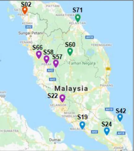
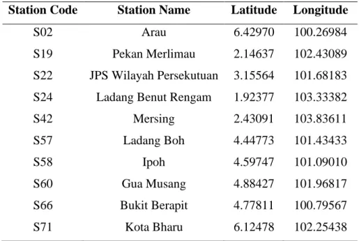
Research Area
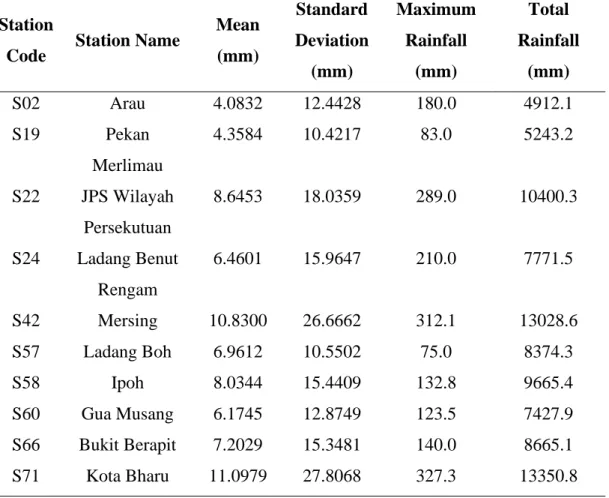
Daily Rainfall Data
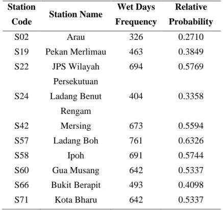
Apart from considering the daily rainfall values, it is also crucial to understand the condition of wet days from the data studied. The frequency of wet days and the relative probability of the occurrence of a wet day are shown in Table 4.03. The Arau station still had the lowest wet day count with the lowest probability of wet day occurrence.
The three stations, Ladang Benut Rengam (S24), Pekan Merlimau (S19), and Bukit Berapit (S66) showed moderate frequency of wet days. The other stations' wet days exceed at least half of the total number of days studied (i.e. 1023 daily observations). Furthermore, the discrepancy between the wet days and the daily rainfall intensities may be due to the increased number of dry days at the end of the NEM season.
As a result, a greater number of dry days were included in the study, reducing the overall frequency of wet days. The highest frequency of wet days can be seen from Ladang Boh Station (S57), which is located at a higher altitude. This resulted in a higher probability of wet days but with low precipitation, corresponding to a minimum maximum precipitation observation of 75.0 mm.
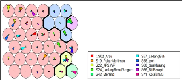
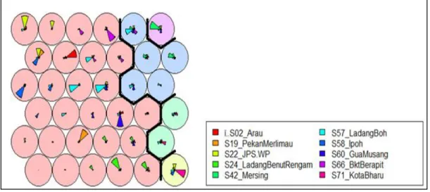
Trained SOFM
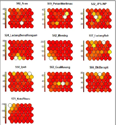
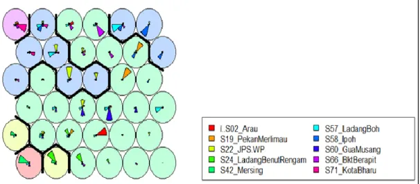
In other words, observations classified in any of the neurons of the same cluster region are believed to share some similarity in terms of the pattern of daily rainfall values. Although boundaries were constructed to obtain the 5 clusters, one can examine that the patterns of rainfall intensities among the rainfall stations illustrated by the colored sectors in the neurons of the three respective Kohonen maps are mostly different from each other. The color filled by the neurons in the heat maps is based on the spectral band that indicates the rainfall intensity.
For example, the white neuron located at (row 5, column 4) of the heat map from Arau station in Figure 4.05 which corresponds to the same neuron position in the Kohonen map in Figure 4.02, indicates the location where observations of the highest rainfall value from Arau -stations will be classified. Again from the heat maps it could be seen that the rainfall stations do not share much similarity in terms of the rainfall pattern. However, it should be noted that the heat maps of the rainfall stations, Mersing (S42) and Kota Bharu (S71) contain observations of high daily rainfall values which are reflected by their wider range of spectral bands.
Both rainfall stations lie on the border of the west coast of Peninsular Malaysia and experience high rainfall intensity associated with strong winds of the northeast monsoon season. The EWM wind may have a weaker influence on other precipitation stations of the western regions due to the existence of many high mountains, such as Since the geographical conditions for the precipitation stations differ considerably from one another, the resulting distribution of precipitation is sparse and uneven.
Performance of the SOFM
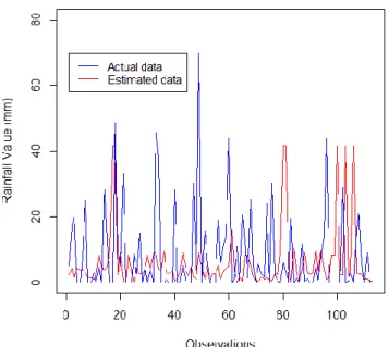
Most of the estimated observations were in good agreement with the actual observations, but there were some fluctuating values for the missing 10% shown in Figure 4.08. There was slightly more evidence of underestimated precipitation observations with larger variations for which the SOFM did not capture the 30% missing proportion illustrated in Figure 4.10. In general, the missing daily precipitation observations that were highly underestimated were those observations with high precipitation values.
In other words, the high peaks seen in the comparison graphs were mostly the ones not captured very accurately by the SOFM model. The primary cause is that the daily precipitation observations that are missing were those of rare and high precipitation values, which had not been taken into account during the training of the SOFM model.
Conclusions
Recommendations
Analysis of climate variability, trends and predictions in the most active parts of the Lake Chad Basin in Africa. Reconstruction of missing daily precipitation data using regression trees and artificial neural networks for SWAT streamflow simulation. A new approach for handling climate missing databases applied to daily rainfall data in the Soummam catchment, Algeria.
Comparative analysis of different techniques for spatial interpolation of precipitation data to create a serially complete monthly time series of precipitation for Sicily, Italy. A simultaneous analysis of climatic trends in several variables: An example of the application of multivariate statistical methods.