image processing and image analysis of defects in

Background

Light field cameras have become widely used due to the development and improvement of light field imaging. According to the research of the Department of Electrical and Electronic Engineering at Yonsei University, a light field camera is used to defend against spoofing face attacks (Kim, Ban, and Lee, 2014).

Figure 1.1: Fundamental of Plenoptic Camera Imaging (Perwass and Wietzke, 2012).

Computer Vision

Image Processing

Deep Learning

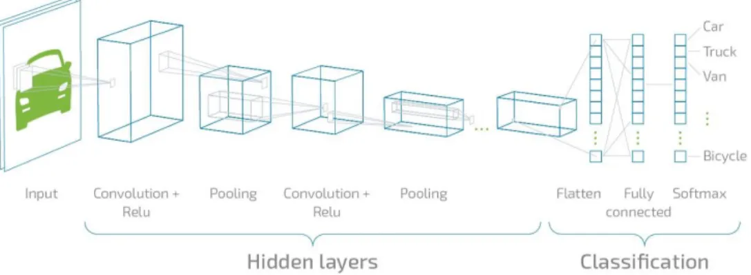
Convolutional Neural Network (CNN)

The RGB image is constructed using three different image planes representing each of the main colors such as red, green and blue. There are two types of pooling as shown in figure 1.6 such as max pooling and average pooling.

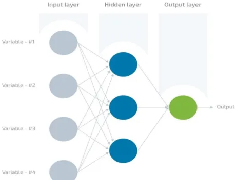
Figure 1.3: The Visualisation of Neural Network (Infopulse, 2019).

Artificial neural network (ANN)

Max Pooling is the process of determining the maximum value of a pixel from part of the image covered by the kernel. On the other hand, the average of all data from the area of the image covered by the kernel is returned by means of average pooling, so that noise can be reduced by reducing dimensionality (Mandal, 2021).

Figure 1.7: A Feed Forward Neural Network with One Hidden Layer (Infopulse, n.d.)

Recurrent Neural Network (RNN)

Problem Statements

Manufacturing defects are a significant factor in degrading the quality of light field images. However, microlens precision management is still difficult due to the fact that the microlens geometry is solely determined by adjusting parameters such as temperature, wettability, pressure, and process time.

Aims and Objectives

Thus, an application that can differentiate the defect status of MLAs if it is. To build a light field imaging system of MLAs to simulate light field imaging with different types of MLA. ii) To design and develop an application that can perform image analysis and image processing on the light field images of MLAs obtained. iii).

Organization of Thesis

Introduction

Camera Calibration

The camera matrix is calculated using a calibration algorithm that uses the generated external and internal parameters. The eigenmatrix and distortion parameters are contained in the camera parameters, which are used to estimate the camera parameters.

Image Processing

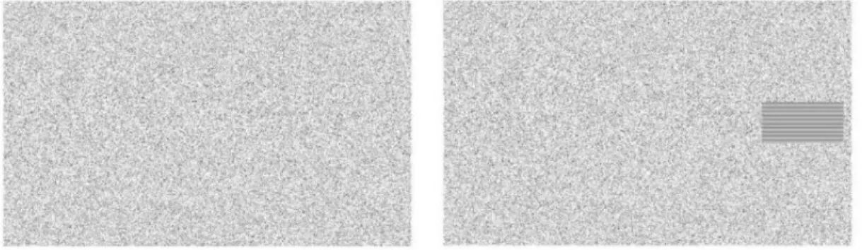
Image Subtraction

Based on Figure 2.3, if the input photos have the same value at a given pixel location, the difference gray value of the image at that point will be zero (black). This method requires the use of a test image 𝑓1(𝑚, 𝑛), and the image must be perfectly aligned with the reference point.

Edge Detection

The performance of edge detection method is highly dependent on the changeable parameters leading to more blurred images. Therefore, to help distinguish real image content from visual artifacts generated by noise, an adaptive edge detection method is required to provide a robust solution that can adjust to the changing noise levels in these images (Bovik and Acton, 2009).

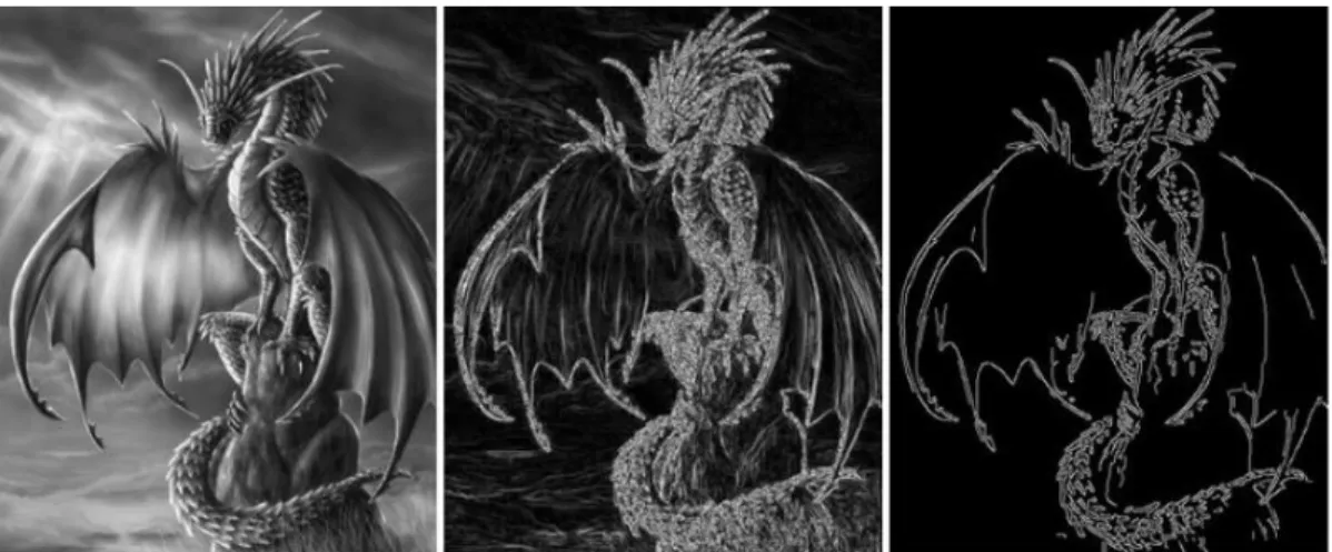
Image Segmentation

Otsu Method

Methods Comparison

Transfer Learning

Pre-Trained Deep Learning Models
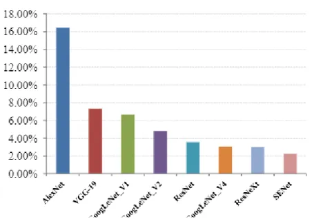
Comparison of Pre-Trained Deep Learning Models
Classification versus One Shot Learning
Datasets

A pre-trained model is one that has already been trained to handle a similar problem by someone else. Even if a pre-trained model is not 100% correct, it saves time and effort from having to start from scratch (Analytics Vidhya, 2017). For example, comparing the pre-trained deep learning models with custom CNN, it is beneficial to use a pre-trained model for various image recognition tasks.

By adopting a pre-trained model, less training and work is required to build the model's architecture. There are several pre-trained models to be selected such as LeNet, AlexNet, VGG, GoogLeNet, Inception V3, Inception BN and so on.

Figure 2.7: Top 5 Error Rate of ImageNet Large Scale Visual Recognition Competition (Itoh et al., 2018)

Methods of Defects Detection on MLAs

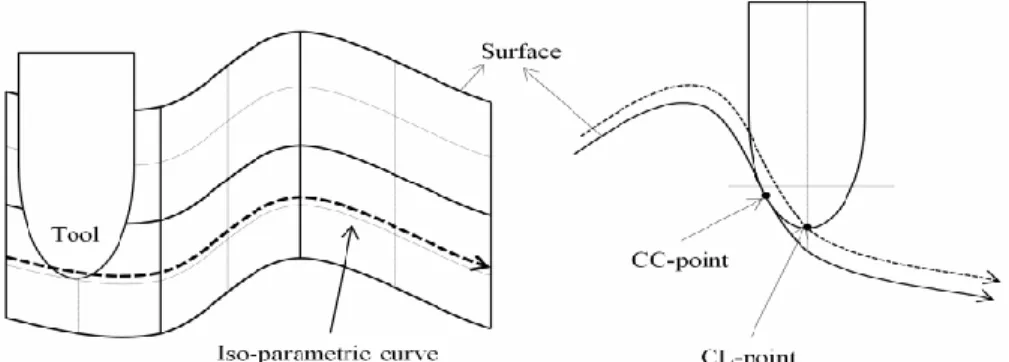
Based on the paper by You and Yang, 2014, a contour error evaluation system was proposed that helps users to select appropriate tool path. Based on Figure 2.13, the quality of an MLA's surface is affected by a variety of factors such as spindle speed, feed rate, tool vibration, heat, tool path data and external environmental factors. Based on Figure 2.14, the process of creating toolpath data for the parametric method and Cartesian method is described.

Despite its drawbacks, the Cartesian technique is often used in real-world environments, due to its ability to compute vehicle path data quickly and its simpler data structure than parametric methods. As a result, in this study, the CL-Cartesian approach was used to produce vehicle path data.

Figure 2.14 Parametric method (Left) Cartesian method (Right) (You and Yang, 2014)

Comparison of the Techniques Used by Other Researchers

With these methods, both the radius of curvature and the focal length of microlenses can be measured without removing the test piece, allowing the results to be compared without confusion over the real lens and without an azimuthal inaccuracy. According to the researchers, there are still areas for improvement, such as improving the interferometer software so that the systematic error of the interferometer can be calibrated to increase measurement accuracy, and the measurements can be automated to enable array testing. In addition, since microlenses are too numerous and small in size, it can be challenging to maintain the surface shape and optical performance of the entire MLA during manufacturing.

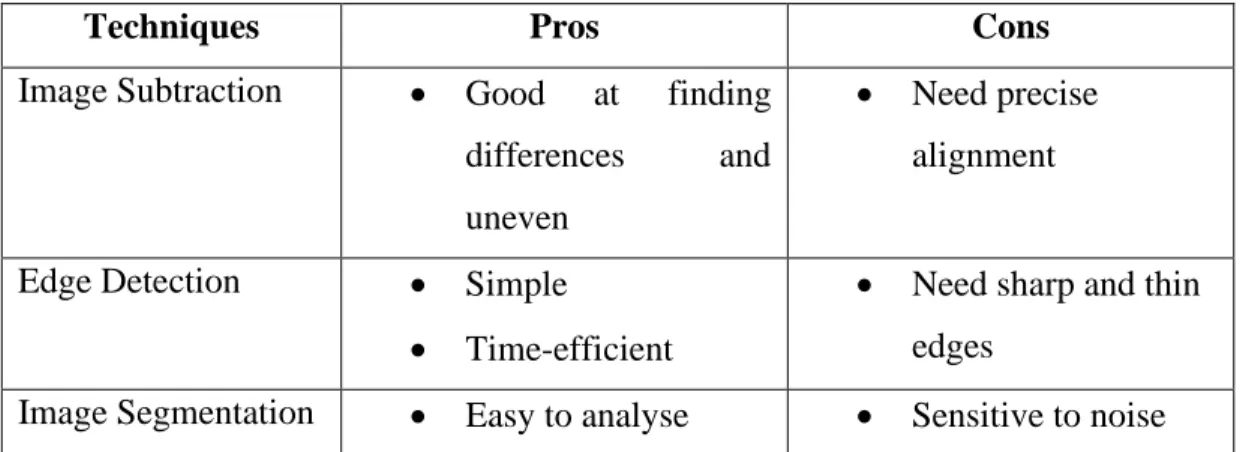
Based on the reviews made in previous research, MLA errors can be categorized into two types such as production error and measurement error. Based on Table 2.3, a comparison was made between all review journals according to techniques, their pros and cons.

System Overview

Equipment

Hardware Configuration

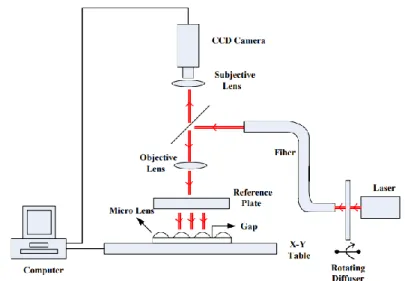
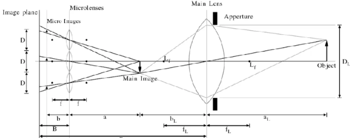
It consists of one Bosch Laser Measure GLM 50 C Professional, VCSEL Lasers Multi-Mode VSCEL Power Array, MLA diffuser and iPhone 13 pro max. From the layout, the MLA diffuser with dimensions of 10cm x 10cm is placed at a distance D=20cm from the camera. As shown in Figure 3.2, there are three different distances, 'd', between the MLA and the MLA diffuser.

MLA with a wavelength of 900 nm is attached to the point where the laser beam is emitted. The Bosch Laser Measure GLM 50 C Professional laser is used as the hardware frame light source to illuminate the MLA surface.

Camera Calibration

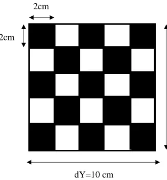
It is treated as the calibration object to calibrate the iPhone 13 pro max camera. The size of the target plate is shown in Figure 3.4, since the MLA diffuser is 10cm x 10cm, a checkerboard image of square sides 10cm each with black and white squares of sides 2cm each is printed and displayed as the calibration pattern. At first, the width and length of the checkerboard are referred to as "dX" and "dY".

The dashboard image is placed on a flat surface parallel to the camera and in the center of the camera's vision as shown in Figure 3.5. With the data image loaded on the laptop, the camera calibration is performed using the camera calibration software shown in Appendix C.

Dataset Preparation and Acquisition

Next, the OpenCV findChessboardCorners() method is used to determine the pixel coordinates (u, v) for each 3D point in the chessboard image. The pixel size of the image is recorded as (dx, dy) for its width and height in pixels respectively. There are three types of MLAs such as Reference, Flat and Narrow that are used to produce light field images, and 10 images are captured for the three types respectively.

Once the image data is recorded, it is uploaded to a desktop computer for further processing via a USB cable, in order to preserve the full resolution of the images. For image processing, images are loaded directly into the software when individual images are selected.

Image Processing Operation

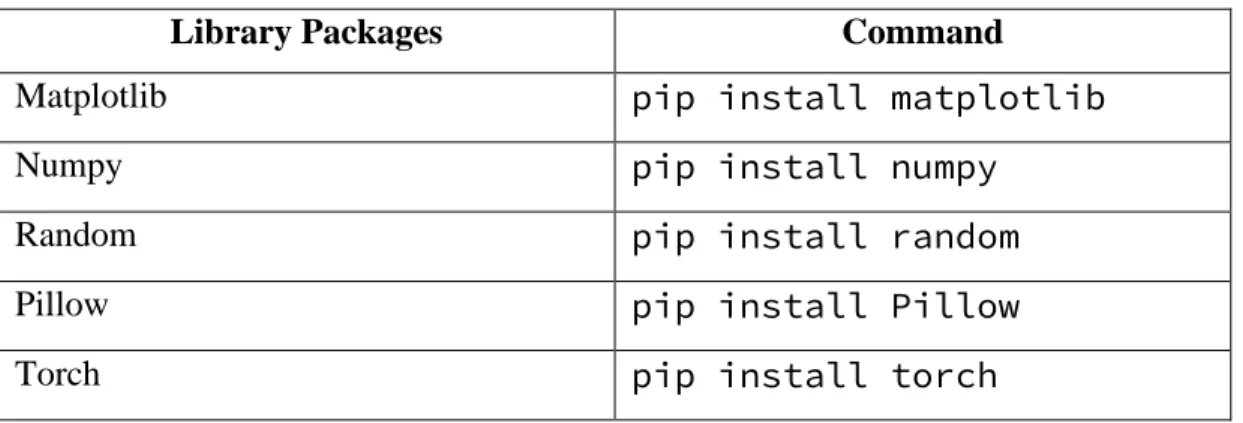
Installation of Required Software and Library Packages

Since the main objective of this project is to detect defects on MLAs, one reference image is captured for each type of the good condition MLA so that comparison can be made to compare between defective MLAs and defect-free MLAs. After annotation, all 30 images of the dataset are equally divided between training, validation and testing, and then exported in PascalVOC format. Before Python language can be used in PyCharm, Python is downloaded and installed from the main Python web page as shown in Figure 3.6.

Therefore, the version of Python 3.9 (64-bit) based on the operating system is downloaded on the laptop used for this project. From the requirement suggested by PyCharm shown in Figure 3.7, the specifications of the laptop used for this project are inspected.

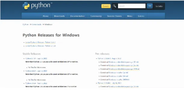
Figure 3.6: Main Webpage for Python Installation.

Image Processing Main Software

Deep Learning Main Software

The dataset exported in PascalVOC format is then used to train the Siamese Neural Network model by uploading the zip file to Google Colaboratory.

Table 3.3 Pip Installation Command for Library Packages.

Cost Analysis of the Project

Project Management

Hardware Testing

Camera Calibration

Camera Calibration (Data Preparation)

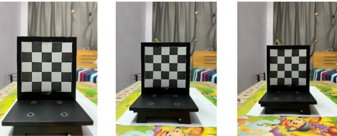
The developed camera calibration system was tested with 6 chessboard images captured from different angles shown in Figure 4.1 and Figure 4.2. Based on Figure 4.3, a snapshot of the results obtained for one of the calibration test images is shown.

Figure 4.2: Checkerboard Images with 20cm, 25cm, 30cm Camera’s Distance (Left to Right)

Camera Calibration (Data Testing)

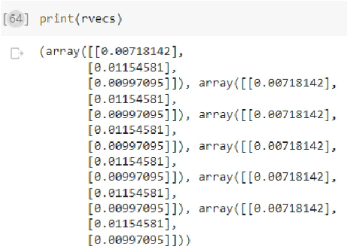
The cv.calibrateCamera() function shown in Figure 4.5 is used to obtain the camera matrix, distortion coefficients, rotation and translation vectors. We then obtain the external matrix of the camera with the rotation matrix, 'R' and the translation vector 't' as shown in equation 4.2. First, the rotation vectors (rvecs), as shown in Figure 4.7, are obtained from the camera calibration system.

Similar to rotation vectors, translation vectors (tvecs), as shown in Figure 4.9, are the result of translating (x, y, z) from the origin. Based on Figure 4.11, the absolute norm between the results of the transformation and the process of locating the corners is determined.

Figure 4.8: Output Messages of Rotation Matrix.

Camera Calibration (Calculations)

Software Testing

Image Processing Based Software Simulation
Deep Learning Based Software Simulation

After the test image is loaded, the path of both the reference image and the test image are displayed in the output messages based on Figure 4.18. From Figure 4.21, the input image is loaded into the system and the Gaussian kernel size is changed. From Figure 4.22, the image type, image shape, image dimensions, maximum RGB value and the center of the image are located.

Based on Figure 4.25, the laser beam profile and intensity distributions of the reference MLA and the reference MLA returned by the hardware configuration are shown. Based on Figure 4.27, the scratch appears as a white dot in the center of the laser beam profile.

Figure 4.21: Input Image, Gaussian Blur Applied Image [5 5] and Gaussian Blur Applied Image [7 7] (Left to Right)

Comparison Between Two Proposed Method

Conclusion

In a nutshell, despite the proposed systems not being tested in the field, the system's performance was assessed, the findings were satisfactory. However, the system still has significant limitations, and those limitations need to be addressed, and some other improvements and changes could be made.

Limitations and Recommendations

Available at: https://www.addoptics.nl/optics-explained/microlens-arrays/#:~:text=Microlens%20arrays%20are%20most%20often [Accessed September 7. Available at: https://instrumental. com/resources/improve-product-quality/machine-vision-vs-manual-inspection-vs-instrumental/ [Accessed 10 Sep