Mean-Variance and Single-Index Model Portfolio Optimisation

(1)

Asian Journal of Business and Accounting 15(2), 2022 79

Mean-Variance and Single-Index Model Portfolio Optimisation:

Case in the Indonesian Stock Market

Adi Kurniawan Yusup*

ABSTRACT

Manuscript type: Research paper

Research aims: This study aims to compare the performance of mean- variance and single-index models in creating the optimal portfolio.

Design/Methodology/Approach: This study creates optimal portfolios using the mean-variance and single-index models with daily stock return data of 38 companies listed on the LQ45 index, IDX Composite index and Bank Indonesia’s 7-Day (Reverse) Repo Rate from January 1, 2012 to December 31, 2019. The two models are compared using the Sharpe ratio.

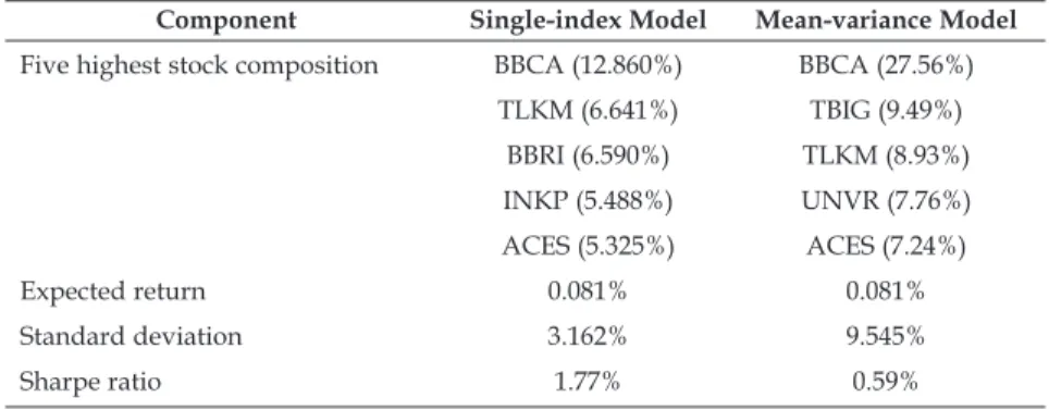
Research findings: The result shows that the single-index model dominates the Indonesian Stock Exchange (IDX), more so than the mean- variance model. BBCA has the highest proportion for both mean-variance and single-index portfolios.

Theoretical contribution/Originality: This study compares two popular portfolio models in the Indonesian stock market.

Practitioner/Policy implication: This study helps investors to create optimal portfolios using a model that is more suited to the IDX.

Research limitation/Implication: This study creates the optimal portfolio without differentiating risk preferences (i.e., risk averse, risk moderate and risk taker). In addition, this research only uses daily return data and does not compare it with weekly and monthly data.

Keywords: Mean-variance Model, Optimal Portfolio, Single-index Model JEL Classification: G11

* Corresponding authors. Adi Kurniawan Yusup is a doctoral degree student of Widya Mandala Catholic University, Surabaya, Indonesia, e-mail: adikurniawanyusup@hotmail.

com

https://doi.org/10.22452/ajba.vol15no2.3

(2)

80 Asian Journal of Business and Accounting 15(2), 2022

1. Introduction

The pandemic created significant problems in the business world.

Most sectors worldwide, including in Indonesia, had to stop their operations temporarily to minimise the spread of Covid-19. The Central Bureau of Statistics of Indonesia reported that the country’s GDP shrank by 5.32% in the second quarter of 2020, 3.49% in the third quarter and 2.19% in the last quarter (Bank Indonesia, 2020).

The Indonesian government rolled out several policies to boost its GDP, including easy fiscal and monetary policies to increase consumption, investment, government spending, and export, as the four components of GDP (Aryusmar, 2020). As a result, many became interested in investing with the relaxation of investment policies. The Indonesia Stock Exchange (IDX) accounted for 3.88 million investors at the end of 2020 (Depository, 2020), and exceeded its annual target of 3 million last year.

Return is one of the factors that motivates investors as a reward for their courage in taking risks. Many investors invest in stocks to get a high return instantly (Hamka et al., 2020). They should use surplus funds after financing their primary need to invest because there is a risk of loss. Moreover, investing in stocks needs long periods to achieve high returns (Partono et al., 2017). However, Indonesia’s Financial Service Authority (2019) showed that financial literacy in the country was at 38.03%, which is considered low.

This is reflected in many using loans and primary-need money for investment. In addition, low financial literacy could increase the information asymmetry that increases herding behaviour (Din et al., 2021), that is, investing is the same stocks as others with the hope of high returns (Fransiska et al., 2018). Nevertheless, this behaviour causes investors to pick the wrong stocks for their portfolio, which leads to losses. Therefore, building an investment portfolio is a critical issue for investors.

Generally, investors are risk-averse (Reilly & Brown, 2003). They expect high returns with low risk, whereas investment theory states that there is a linear relationship between risk and return, i.e., high risk, high return (Rui et al., 2018). Hence, risk should be reduced to get the desired return with lower risk. A fundamental approach to minimising risk is diversification (Lee et al., 2020). Diversification is the allocation of a fixed portfolio across different types of securities and asset classes that limit exposure to any source of risk (Bodie et al., 2014). The optimal portfolio for the most returns with the lowest risk is located in the efficient frontier curve (Fama & French, 2004).

However, creating an optimal portfolio is a challenge, especially

(3)

Asian Journal of Business and Accounting 15(2), 2022 81 for new investors. Investors need to work with a lot of information, e.g., historical price, trends and firm performance. They also need analytical tools to get the right composition of stocks in their portfolio.

One approach used to obtain an optimal portfolio is modern portfolio theory (MPT) or mean-variance analysis. MPT was established by Markowitz (1952), and attempts to maximise portfolio return for any given risk, or equivalently, minimise risk for any given amount of return. Both ways will produce the same result in creating an efficient portfolio. The basic concept behind MPT is that assets in a portfolio should not be viewed in isolation but should be evaluated by how it affects the portfolio’s risk and return on the whole (Omisore et al., 2012). MPT seeks to reduce total variance as a component of risk of portfolio return by combining different assets with returns that are not positively correlated. This theory assumes that investors are rational and markets are efficient.

The Markowitz model provides several risk-return combinations which investors can choose from based on their preferences (Putra &

Dana, 2020; Rigamonti, 2020). However, implementing the Markowitz model is very time-consuming, because it requires a lot of estimations to fill the covariance matrix. The model does not provide guidelines for forecasting the security risk premium, that is important for the construction of an efficient frontier of risky assets (Singh & Gautam, 2014). Sharpe (1963), in trying to simplify the Markowitz model, came up with a single-index model that reduces computational requirements and data. This model solves the portfolio optimisation problem by showing a linear relationship between risk and return—

which is simpler to understand—and considers that the relationship between securities occurs only through their individual relationship with some indices of business activity. As a result, covariance data is reduced from (n² – n)/2 under the Markowitz model to only n measures of each security as it relates to the index (Chitnis, 2010).

Nevertheless, single-index models may not be the most efficient with respect to volatility.

There are limited studies on comparing the mean-variance and single-index models in creating a portfolio. Furthermore, those studies show inconsistent results. Ozkan and Cakar (2020) show that the mean-variance model performs better in the markets of developed countries, while the single-index model performs better in developing countries. On the other hand, Chasanah et al. (2017), whose research sample is a developing country market, find that optimal portfolio formation with the mean-variance model is more dominant than the

(4)

single-index model. Nyokangi (2016) shows that the choice between mean-variance and single-index models depends on the time span of study. On the other hand, Yuwono and Ramdhani (2017) find no significant return difference between the mean-variance model and single-index model.

Therefore, this paper aims to construct portfolios using the mean- variance and single-index models, and compare the performance of each in the IDX. The sample used in this research are stocks listed in the LQ45 index, the most liquid stocks in the IDX. This research is expected to give insight to investors—especially new investors—on constructing an optimal portfolio.

2. Literature Review

2.1 Portfolio Theory (Markowitz Theory)

Asset allocation for the sake of diversification in financial markets has become an important issue for investors. Investors expect asset allocation to give them the highest return with a particular risk, or the lowest with a certain expected return. Diversification is a risk reduction technique by spreading investment in different securities and asset classes (Bodie et al., 2014; Jayeola et al., 2017). In the traditional approach of diversification, the greater the number of securities invested in portfolio, the lower the risk (Lekovic, 2018).

Based on the law of large numbers, this theory is supported by some its proponents, like Hicks (1935), Williams (1938), and Leavens (1945). Nevertheless, portfolio efficiency decreases as the number of portfolios increases because it results in excessive diversification. This can reduce portfolio risk, but ignores the correlation between returns on different assets (Francis & Kim, 2013).

Simple diversification was rejected by Markowitz (1952), who was awarded the Nobel Prize in 1990 for his essay “Portfolio Selection” and his book Portfolio Selection: Efficient Diversification (1959). He initiated the first quantitative theory of portfolio selection and management, currently known as MPT. This is a framework to create an investment portfolio based on the maximisation of expected returns and the simultaneous minimisation of investment risk (Fabozzi et al., 2002; Rodríguez et al., 2021). This theory uses return and risk in a coherent framework (Chen & Pan, 2013) and considers covariances among the stocks in the portfolio. This model is also called the mean-variance (MV) portfolio theory. Return is based on historical data while risk is obtained from standard deviation of returns. The Markowitz model provides a solution to

(5)

Asian Journal of Business and Accounting 15(2), 2022 83 overcome trade-off problems between risk and return in selecting a combination of assets in an optimal portfolio. The investor has a choice of either maximising return with any acceptable risk or to minimise risk with any acceptable level of return. Both options use the same mathematical process.

Efficient frontier refers to several alternative portfolios that give the highest return on certain risks or lowest risk on certain returns (Fabozzi et al., 2002; Letho et al., 2022). Nevertheless, not all portfolios on the efficient frontier are optimal. An optimal portfolio is located on the efficient frontier chosen by investors based on their individual preferences shown by utility. Theoretically, an optimal portfolio is defined as a tangency point between the efficient frontier and the investor’s indifference curve, which presents the utility of the investor. A higher indifference curve has larger certainty equivalents and larger expected utility (N. Kumar, et al., 2014).

However, this theory has several limitations. Mean-variance portfolios find portfolio weight based on first moment and the parametric representation of second moment, assuming no predictable time variation. It assumes constant investment opportunities, and its static mean-variance solution is myopic and does not consider events beyond the present (Jones, 2017). MPT also assumes continuous pricing, a world in which markets are free, societies are stable, and investors are rational wealth maximisers (Curtis, 2004). In fact, this assumption is contradicted by observations of investors who get swept up in herd behaviour, whereby the investor tries to follow the decisions made by others and undervalues information available in the market (Bikhchandani & Sharma, 2000).

They do not consider risk and return in choosing their portfolio.

Moreover, these models need complex statistics-based mathematical modelling and formulas to support the concept and theoretical assumptions (Mangram, 2013). This is problematic when it is used to build portfolios from large stock groups, with many estimations needed for asset selection.

2.2 Single-index Model

The single-index model (SIM) concept was developed by Sharpe in 1963. This model simplifies Markowitz’s mean-variance model (Mahmud, 2019) to overcome its complexity. This model is no longer based on inter-asset correlation, but instead on the assumption that co-movement between stock return is due to movement in market returns, or to be more specific, returns of a broad market index, R_M (Frankfurter et al., 1976; Hadiyoso et al., 2015). The single-index

(6)

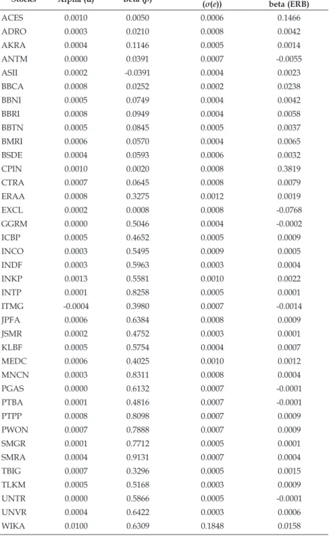
model specifies two sources of uncertainty for return: systematic and unique uncertainty. Systematic uncertainty, or beta (β), is uncertainty from the market or macroeconomics, while unique uncertainty, alpha (α), is uncertainty from the company or industry itself. Hence, a single-index model is written as follows:

i i i M

R = + a b R + e

From the equation, the difference between expected return (a_i + b_iR_M) and actual return (R_i) is symbolised by e,, residual return.

An important concept in the single-index model is β terminology.

This refers to sensitivity towards market return and is usually predicted using historical data (B. R. Kumar & Fernandez, 2019).

The higher the β, the more sensitive the stock is to market return.

The basic assumption used in the single-index model is that stocks are correlated only if they have the same response toward market return. Therefore, the covariance between two stocks only can only be calculated based on the similarity of their response toward market returns.

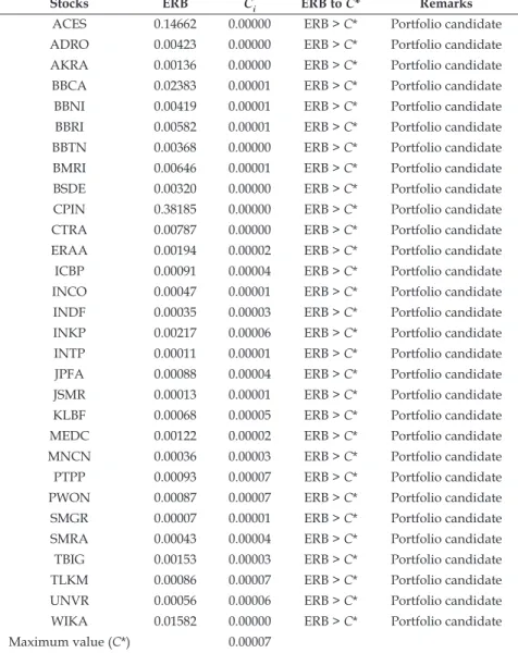
The optimal portfolio of the single-index model is obtained by sorting the value of excess return to β (ERB) for each stock from the largest to the smallest (Elton et al., 1976). The negative ERB value or positive ERB that is caused by negative excess return and negative β has to be removed. Those ERB values are compared with the value of cut-off point of the shares (C*). C* is the largest value C_i of each individual stock. Stocks with larger ERB value compared to the C*

are included in the optimal portfolio and the weights are calculated, while others are taken out.

3. Methodology

3.1 Database

This research uses daily closing prices of stocks incorporated in the LQ45 index, IDX Composite index and Bank Indonesia’s 7-Day (Reverse) Repo Rate (7-DRRR), from January 2012 to December 2019.

LQ45 represents the 45 most liquid companies on the IDX based on the following criteria: highest capitalisation, huge transaction value and prospects for future growth (Malini, 2019). The annual closing price of stocks are gathered from Yahoo Finance, then matched with financial statement reports from IDX. The IHSG index is obtained from Yahoo Finance, and the risk-free rate date is obtained from Bank

(7)

Asian Journal of Business and Accounting 15(2), 2022 85 Indonesia’s 7-DRRR report.

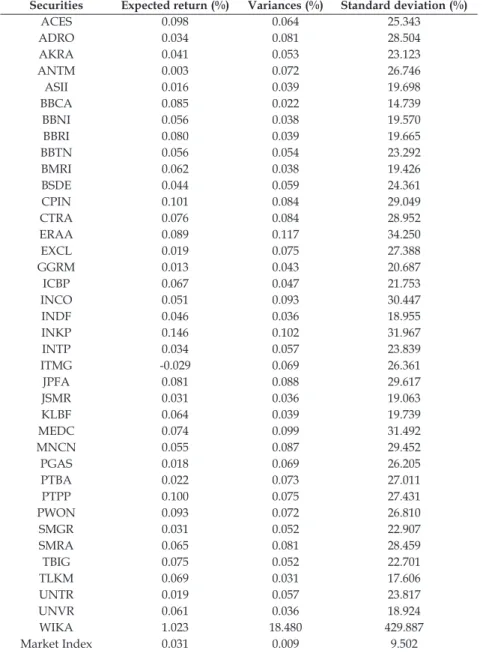
A total of 38 companies on the LQ45 index are used as the research sample. These are the only firms on the LQ45 index with enough information in the examined period. The other seven LQ45 companies do not have complete data—some issued stocks after 2012, and some had their stocks suspended, resulting in no trade for several days. When those stocks were traded again, the price could differ significantly from the last trading period, showing high volatility (Garcíaa et al., 2015). These 38 companies comprise various sectors, as listed in Appendix 1.

3.2 Research Procedure

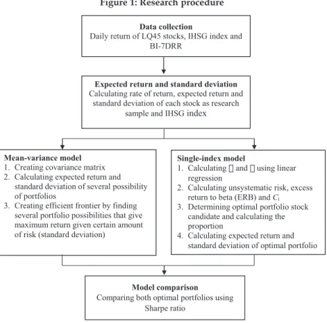
Figure 1 shows the steps of constructing a portfolio using both the mean-variance and single-index models and comparing the results.

Figure 1: Research procedure

7

Figure 1: Research procedure

3.3 Expected Return and Standard Deviation of Individual Stock

The expected return of individual stock is the arithmetic mean of daily return during the research period (Benniga, 2006) as follows:

𝐸𝐸(𝑅𝑅𝑖𝑖) =∑𝑘𝑘 𝑅𝑅𝑖𝑖

𝑖𝑖=1𝑘𝑘 (1)

Where:

Rate of return of stock i k Number of rate of return data

Expected return of stock i

Ri

( )_i E R

Data collection

Daily return of LQ45 stocks, IHSG index and BI-7DRR

Expected return and standard deviation Calculating rate of return, expected return and

standard deviation of each stock as research sample and IHSG index

Mean-variance model 1. Creating covariance matrix 2. Calculating expected return and

standard deviation of several possibility of portfolios

3. Creating efficient frontier by finding several portfolio possibilities that give maximum return given certain amount of risk (standard deviation)

Single-index model

1. Calculating and using linear regression

2. Calculating unsystematic risk, excess return to beta (ERB) and Ci

3. Determining optimal portfolio stock candidate and calculating the proportion

4. Calculating expected return and standard deviation of optimal portfolio

Model comparison

Comparing both optimal portfolios using Sharpe ratio

(8)

3.3 Expected Return and Standard Deviation of Individual Stock The expected return of individual stock is the arithmetic mean of daily return during the research period (Benniga, 2006) as follows:

7

Figure 1: Research procedure

3.3 Expected Return and Standard Deviation of Individual Stock

The expected return of individual stock is the arithmetic mean of daily return during the research period (Benniga, 2006) as follows:

𝐸𝐸(𝑅𝑅𝑖𝑖) =∑𝑘𝑘 𝑅𝑅𝑖𝑖 𝑖𝑖=1

𝑘𝑘 (1)

Where:

Rate of return of stock i k Number of rate of return data

Expected return of stock i

R

i

( )

_i

E R

Data collection

Daily return of LQ45 stocks, IHSG index and BI-7DRR

Expected return and standard deviation Calculating rate of return, expected return and

standard deviation of each stock as research sample and IHSG index

Mean-variance model 1. Creating covariance matrix 2. Calculating expected return and

standard deviation of several possibility of portfolios

3. Creating efficient frontier by finding several portfolio possibilities that give maximum return given certain amount of risk (standard deviation)

Single-index model

1. Calculating and using linear regression

2. Calculating unsystematic risk, excess return to beta (ERB) and Ci

3. Determining optimal portfolio stock candidate and calculating the proportion

4. Calculating expected return and standard deviation of optimal portfolio

Model comparison

Comparing both optimal portfolios using Sharpe ratio

(1)

Where:

R_i Rate of return of stock i k Number of rate of return data E(R_i) Expected return of stock i

Variances and standard deviation measure the risk of an individual stock. Variance measures the averaged squared difference between actual and average return, while standard deviation is the square root of variance (Bradford & Miller, 2009). Larger variances and standard deviation indicate greater volatility. Variance and standard deviation are calculated as follows:

2 ^k1( i ( ))i (2)

i i

R E R

s ⁼ -k

=

å

(2)

(3)

i 2i

s = s ⁽³⁾

Where:

R_i Rate of return of stock i k Number of rate of return data E(R_i) Expected return of stock i S ² Variances of stock i ⁱ

S_i Standard deviation of stock i

3.4 Mean-variance Model 3.4.1 Creating Covariance Matrix

Covariance measures how returns on two risky assets move in tandem (Bodie et al., 2014). If the covariance is positive, two assets move together while they vary inversely if the covariance is negative.

Covariance is calculated as follows:

(9)

Asian Journal of Business and Accounting 15(2), 2022 87 Pr( )[ ( )][ ( )] (4)

ij i i j j

scenarios

scenario R E R R E R

s =

å

- - ⁽⁴⁾

Total covariance data =

Total covariance data = (5)

2

n - n ₂

i i

s = s ⁽⁵⁾

Where:

R_i Rate of return of stock i E(R_i) Expected return of stock i R_j Rate of return of stock j S_ij Covariance of stock i and j

n Number of stocks as sample

The covariance matrix is a tool to calculate the standard deviation of a stock portfolio that is used to quantify risk. The format of the covariance matrix is as follows:

Covariance matrix =

1

2

2 1 2 1

2 2

1 2

1 2 2

var cov( , ) cov( , )

cov( , ) var cov( , )

...

cov( , ) cov( , ) ... var ù

é ú

ê ú

ê û

ë ⁿ

x n

n

x x x x

x x x

x

x x x x

(6)

3.4.2 Calculating Expected Return and Standard Deviation of Portfolio

The expected return of portfolio is the weighted average of individual stock return (Rachmat & Nugroho, 2013) and can be calculated using the following expression.

(7)

1

( ) ( )

=

å

ⁿ

P i i

i

E R w E R (7)

Where:

R_i Rate of return of stock i

E(R_p) Expected return on the portfolio w_i Weight of stock i in the portfolio n Number of stocks included in portfolio E(R_i) Expected return of individual stock i

Risk in portfolio management is measured through uncertainty of the returns. Correlation, coefficients, weights of each security and variance of its stocks are factors influencing portfolio risk (Aliu et al., 2017). Risk can be divided into two types: systematic risk (market

(10)

risk or non-diversifiable risk) and unsystematic risk (diversifiable risk) (Wagdi & Tarek, 2019). Risk of the portfolio proxied by standard deviation can be calculated as follows:

2 (8)

1 1

n n

p i j ij

i j

w w

s s

= =

=

å å

⁽⁸⁾

^s^p⁼ ^s²^p ⁽⁹⁾ ⁽⁹⁾

Where:

s

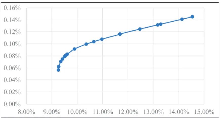
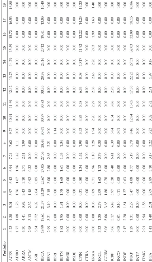
²_p Variance of the portfolio Variance of the portfolio w_i Weight of stock i in the portfolio w_j Weight of stock j in the portfolio n Number of stocks included in portfolio S_ij Covariance between stock i and stock j S_p Standard deviation of portfolio 3.4.3 Creating Efficient Frontier Curve

An approach used in this research to find optimal portfolios located in efficient frontier curve is generating portfolio with maximum return for any given standard deviation.

10

(8) (9) Where:

Variance of the portfolio wi Weight of stock i in the portfolio wj Weight of stock j in the portfolio n Number of stocks included in portfolio

Covariance between stock i and stock j Standard deviation of portfolio

3.4.3 Creating Efficient Frontier Curve

Max (10)

Some restrictions used to find Max are as follows:

Given standard deviation: (11)

1. (12)

2. (13)

(no short position is available) 3.5 Single-index Model

3.5.1 Calculating and Using Linear Regression

To find and for each stock in single-index model, we regress the return of each stock on the market return. The regression equation is as follows:

2

1 1

n n

p i j ij

i j

w w

s s

= =

=

å å

p 2p

s = s

2p

s

ij

s

p

1

( )_P ⁿ _i ( )_i

i

E R w E R

=

å

( )

_P

E R

1 1

n n

p i j ij

i j

w w

s s

= =

=

å å

1 n 100%

i i

w

=

å

=

i

0 w ³

(10)

Some restrictions used to find Max E(R_p) are as follows:

Given standard deviation:

10

(8) (9) Where:

Variance of the portfolio wi Weight of stock i in the portfolio w^j Weight of stock j in the portfolio n Number of stocks included in portfolio

Max (10)

1. (12)

2. (13)

2

1 1

n n

p i j ij

i j

w w

s s

= =

=

å å

p 2p

s = s

2p

s

ij

s

p

1

( )_P ⁿ _i ( )_i

i

E R w E R

=

å

( )

_P

E R

1 1

n n

p i j ij

i j

w w

s s

= =

=

å å

1 n 100%

i i

w

=

å

=

i

0 w ³

(11)

1.

10

(8) (9) Where:

Max (10)

1. (12)

2. (13)

2

1 1

n n

p i j ij

i j

w w

s s

= =

=

å å

p 2p

s = s

2p

s

ij

s

p

1

( )_P ⁿ _i ( )_i

i

E R w E R

=

å

( )

_P

E R

1 1

n n

p i j ij

i j

w w

s s

= =

=

å å

1 n 100%

i i

w

=

å

=

i

0 w ³

(12) 2.

10

(8) (9) Where:

Max (10)

1. (12)

2. (13)

2

1 1

n n

p i j ij

i j

w w

s s

= =

=

å å

2

p p

s = s

2p

s

ij

s

p

1

( )_P ⁿ _i ( )_i

i

E R w E R

=

å

( )

_P

E R

1 1

n n

p i j ij

i j

w w

s s

= =

=

å å

1 n 100%

i i

w

=

å

=

i

0 w ³

(13)

(no short position is available)

(11)

Asian Journal of Business and Accounting 15(2), 2022 89 3.5 Single-index Model

3.5.1 Calculating α and β Using Linear Regression

To find α and β for each stock in single-index model, we regress the return of each stock on the market return. The regression equation is as follows:

(14)

i i i M

R = + a b R + e

(14)

Where:

R_i Return of a stock R_M Market return

αi Individual stock’s alpha (intercept), part of return that is not affected by market

β_i Individual stock’s beta (slope), part of return that is affected

by market

e Residual

3.5.2 Calculating Unsystematic Risk, Excess Return to Beta (ERB) and Ci Unsystematic risk is risk specific to individual company (firm-specific risk) (Masry & Menshawy, 2017). There are two methods to calculate unsystematic risk: direct and indirect. Using the direct method, unsystematic risk uses residuals of a factor model, such as CAPM and the Fama and French (1993) model. Using the indirect method, unsystematic risk can be calculated using the following formula:

Unsystematic risk = Total risk – systematic risk (15) (16)

2

( ) e

_i _i2 _i2 2_M

s = - s b s

(16)

Where:

s

²

( ) e

_i Unsystematic risk of stock

= - s

_i²

b s

_i^{2 2}_M i (16)

(16)

2

( ) e

_i _i2 _i2 2_M

s = - s b s

Variances (total risk) of stock i ² Beta square of stock i

b

i Beta square of stock i

s

²M Variances of market index Variances of market index

Excess return is the difference between stock return and the risk- free rate. In this case, the risk-free rate is 7-DRRR. Excess return to beta (ERB) measures the relative premium return of a stock toward unit risk that could not be diversified. ERB is calculated as follows:

(12)

(17) ( )_i _f

i

E R R

ERB b

= -

(17)

Where:

E(R_i) Expected return of stock i R_f Risk-free rate

b_i Beta of stock i

ERB_i Excess return to beta of stock i

To determine which stocks are included in a portfolio, the cut-off point (C*) has to be determined. The cut-off point value is obtained from the highest amount of C_i of each individual stock. C_i is calculated as follows:

2 2

1

2 2

1 2

[ ( ) ] ( )

1 ( )

n i f i

M i i

i

n i

M i i

E R R

C e

e s b

s s b

s

=

-

= æ ç ö ÷

+ ç ÷

ç ÷ ç ÷

è ø

å å

(18)

Where:

² ²

1

2 2

1 2

[ ( ) ] ( )

1 ( )

n i f i

M i i

i

n i

M i i

E R R C e

e s b

s s b

s

=

-

= æ ç ö ÷

+ ç ÷

ç ÷ ç ÷

è ø

å å

Variances of market E(R_i) Expected return of stock i R_f Risk-free rate

b_i Beta of stock i

S²(e_i) Unsystematic risk of stock i

3.5.3 Determining Optimal Portfolio Stock Candidate and Calculating Proportion

The prerequisite of a stock included into an optimal portfolio is that its ERB value is higher than C* which can be written as follows:

(19)

i *

ERB C> (19)

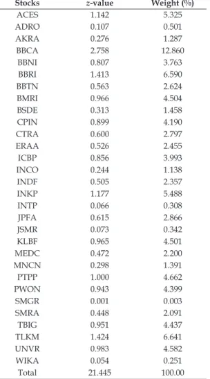
Among all stocks that fulfil criteria (19), we have to calculate z-value to determine the stock weight in the optimal portfolio. The formula to calculate z-value with no short position available is as follows:

(13)

Asian Journal of Business and Accounting 15(2), 2022 91

13

(20)

Where:

Z-value of stock i Beta of stock i

Unsystematic risk of stock i ERBi Excess return to beta of stock i C* Cut-off point (maximum value of Ci)

Based on those z-values, the proportion of each stock in optimal portfolio can be calculated as:

(21)

Where:

wi Weight of stock i in optimal portfolio S-value of stock i

n Number of stocks that meet criteria (19)

The expected return of portfolio using the single-index model is calculated using the following equation:

(22) Where:

Expected return of portfolio Portfolio alpha that is obtained from

Portfolio beta that is obtained from

Expected market return

2 ( *)

( )ⁱ

i i

i

z ERB C

e b

= s -

z

i

b

i 2

( ) e

_i

s

1

i n i

i i

w z

z

=

å

z

i

( )

_p _p _p

( )

_M

E R = + a b E R ( )

_p

E R a

p

1 n

p i i

i

w

a a

=

å

b

p

1 n

p i i

i

w

b b

=

å

( )

_M

E R

(20)

Where:

Z_i Z-value of stock i b_i Beta of stock i

13

(20)

Where:

(21)

Where:

(22) Where:

2 ( *)

( )ⁱ

i i

i

z ERB C

e b

= s -

z

i

b

i 2

( ) e

_i

s

1

i n i

i i

w z

z

=

å

z

i

( )

_p _p _p

( )

_M

E R = + a b E R ( )

_p

E R a

p

1 n

p i i

i

w

a a

=

å

b

p

1 n

p i i

i

w

b b

=

å

( )

_M

E R

Unsystematic risk of stock i ERB_i Excess return to beta of stock i C* Cut-off point (maximum value of C_i)

13

(20)

Where:

(21)

Where:

(22) Where:

Expected return of portfolio Portfolio alpha that is obtained from Portfolio beta that is obtained from

2 ( *)

( )ⁱ

i i

i

z ERB C

e b

= s -

z

i

b

i 2

( ) e

_i

s

1

i n i

i i

w z

z

=

å

z

i

( )

_p _p _p

( )

_M

E R = + a b E R ( )

_p

E R a

p

1 n

p i i

i

w

a a

=

å

b

p

1 n

p i i

i

w

b b

=

å

( )

_M

E R

(21)

Where:

w_i Weight of stock i in optimal portfolio Z_i S-value of stock i

13

(20)

Where:

Unsystematic risk of stock i ERBⁱ Excess return to beta of stock i C* Cut-off point (maximum value of Ci)

(21)

Where:

(22) Where:

2 ( *)

( )ⁱ

i i

i

z ERB C

e b

= s -

z

i

b

i 2

( ) e

_i

s

1

i ni

i i

w z

z

=

å

z

i

( )

_p _p _p

( )

_M

E R = + a b E R ( )

_p

E R a

p

1 n

p i i

i

w

a a

=

å

b

p

1 n

p i i

i

w

b b

=

å

( )

_M

E R

(22) Where:

E(R_p) Expected return of portfolio

a_p Portfolio alpha that is obtained from

13

(20)

Where:

(21)

Where:

(22) Where:

Portfolio beta that is obtained from Expected market return

2 ( *)

( )ⁱ

i i

i

z ERB C

e b

= s -

z

i

b

i 2

( ) e

_i

s

1

i n i

i i

w z

z

=

å

z

i

( )

_p _p _p

( )

_M

E R = + a b E R ( )

_p

E R a

p

1 n

p i i

i

w

a a

=

å

b

p

1 n

p i i

i

w

b b

=

å

( )

_M

E R

b_p Portfolio beta that is obtained from

13

(20)

Where:

(21)

Where:

(22) Where:

2 ( *)

( )ⁱ

i i

i

z ERB C

e b

= s -

z

i

b

i 2

( ) e

_i

s

1

i n i

i i

w z

z

=

å

z

i

( )

_p _p _p

( )

_M

E R = + a b E R ( )

_p

E R a

p

1 n

p i i

i

w

a a

=

å

b

p

1 n

p i i

i

w

b b

=

å

( )

_M

E R

E(R_M) Expected market return

Portfolio risks consist of systematic risk and unsystematic risk.

Therefore, total portfolio variance is the sum of systematic and unsystematic risk.

Portfolio risk = Systematic risk + Unsystematic risk (23)

14

Portfolio risks consist of systematic risk and unsystematic risk. Therefore, total portfolio variance is the sum of systematic and unsystematic risk.

Portfolio risk = Systematic risk + Unsystematic risk

(23)

Where:

Portfolio variance

Portfolio beta that is obtained from Variances of market

Portfolio unsystematic risk that is obtained from

3.6 Model Comparison

Two optimal portfolios, using the mean-variance and single-index models, with the same expected returns are compared using the Sharpe ratio. The Sharpe ratio is commonly used to measure portfolio performance (Zakamulin, 2008). This ratio is computed as the excess return relative to the risk-free rate divided by risk adjustment by using asset return volatility (Gatfaoui, 2009). The higher the Sharpe ratio is, the better performing the portfolio is.

Sharpe ratio = (23)

Where:

expected return of portfolio risk-free rate

standard deviation of portfolio

Suppose the Sharpe ratio of mean-variance model is higher than single-index model. In that case, it is concluded that the mean-variance model dominates the Indonesian stock market more so than the single-index model. On the contrary, if the Sharpe ratio of the single-index model is higher than the mean-variance model, it dominates the IDX more than the mean- variance model.

2 2 2 2( )

P p M ep

s = b s +s

2P

s b

p

1 n

p i i

i

w

b b

=

å

M2

s

2( )e_p

s ² ²

1

( )_p ⁿ _i ( )_i

i

e w e

s s

=

å

( )_p _f

P

E R R

s -

( )

_p

E R R

F

s

P