i
Amplifier and Filter for Geophone Sensitivity Studies
by
Ainul Shazwanie Binti Mohd Nizam 18185
Dissertation submitted in partial fulfilment of the requirements for the
Bachelor of Engineering (Hons) (Electrical and Electronics Engineering)
JANUARY 2017
Universiti Teknologi PETRONAS, 32610, Bandar Seri Iskandar, Perak Darul Ridzuan.
ii
CERTIFICATION OF APPROVAL
Amplifier and Filter for Geophone Sensitivity Studies by
Ainul Shazwanie Binti Mohd Nizam 18185
A project dissertation submitted to the Electrical and Electronics Engineering Programme
Universiti Teknologi PETRONAS in partial fulfilment of the requirement for the
BACHELOR OF ENGINEERING (Hons)
(ELECTRICAL AND ELECTRONICS ENGINEERING)
Approved by,
_____________________
(Dr. Dennis Ling)
UNIVERSITI TEKNOLOGI PETRONAS BANDAR SERI ISKANDAR, PERAK
January 2017
iii
CERTIFICATION OF ORIGINALITY
This is to certify that I am responsible for the work submitted in this project, that the original work is my own except as specified in the references and acknowledgements, and that the original work contained herein have not been undertaken or done by unspecified sources or persons.
________________
AINUL SHAZWANIE BINTI MOHD NIZAM
iv
ABSTRACT
A geophone is a device that response to the velocity of the ground by the movement of the magnetic mass back and forth to produce a voltage. Generally, geophone can measures a various frequencies of seismic events but there is a limit of frequency that frequencies should be over to get an accurate measurement. The limit is also resonant frequency which is usually in range 4.5Hz to 10Hz depending on the seismic sensor type. If the frequencies detected is below the geophone’s resonant frequency, geophone encounter inaccuracy in detecting the motion. By utilizing a feedback and filter circuits, the sensor can measures even the low frequencies. This will be assessed with a shaking table that is set to a certain frequencies and the measurement of the output can be taken. The aftereffect of the geophone connected with the filter circuits connected to an oscilloscope will be contrasted with the outcomes of the geophone using current geophone circuit. The project of building of the circuit is to enhance the sensitivity of the geophone in detecting lower frequency below resonant frequency.
v
ACKNOWLEDGEMENT
First of all, I would like to express my gratitude and a very special thanks to my supervisor, Dr. Dennis Ling, who was abundantly helpful with the constant guidance and support throughout my research. His guidance helped me to understand better and learn something new apart from my studies in Electrical and Electronics Engineering in Universiti Teknologi PETRONAS.
Other than that, I want to thank to lecturers from Electrical and Electronics Engineering Department as well whom indirectly taught and gave me guidance to complete and prepare my project.
Last but not least, greatest gratitude to my beloved parents and family members who give me endless support and motivation to me throughout the duration of my studies.
vi
TABLE OF CONTENTS
CERTIFICATION OF APPROVAL ... ii
CERTIFICATION OF ORIGINALITY ... iii
ABSTRACT ... iv
ACKNOWLEDGEMENT ...v
CHAPTER 1 ... 1
INTRODUCTION ... 1
1.1 BACKGROUND ... 1
1.2 PROBLEM STATEMENT ... 2
1.3 OBJECTIVE ... 2
1.4 SCOPE OF STUDY ... 2
CHAPTER 2 ... 4
LITERATURE REVIEW ... 4
2.1 GEOPHONE ... 4
2.1.1 ELECTROMAGNETIC PRINCIPLE ... 5
2.2 GEOPHONE CIRCUIT ... 7
2.3 LOW LEVEL FREQUENCY DETECTION ... 8
2.4 AMPLIFIER AND FILTER ... 9
CHAPTER 3 ... 10
METHODOLOGY ... 10
3.1 PROJECT FLOW CHART ... 10
3.2 PROJECT INITIALIZATION ... 11
3.3 PROJECT DEVELOPMENT ... 12
3.3 TOOLS AND EQUIPMENT ... 13
3.4 GANTT CHART AND MILESTONE ... 14
CHAPTER 4 ... 16
RESULTS AND DISCUSSION ... 16
4.1 GEOPHONE EQUIVALENTS ... 16
4.2 CIRCUITRY DESIGN ... 19
4.3 EXPERIMENTAL RESULT ... 20
CHAPTER 5 ... 28
CONCLUSION AND RECOMMENDATION ... 28
5.1 CONCLUSION ... 28
vii
5.2 RECOMMENDATION ... 29
REFERENCES ... viii
APPENDIX 1 ... x
APPENDIX 2 ... xi
TABLE OF FIGURES
Figure 1 Mechanical design of geophone ... 4Figure 2 Geophone damping resistor circuit ... 7
Figure 3 Geophone element connected with the damping resistor ... 7
Figure 4 Sensitivity curve of geophone operated in open circuit condition and closed system with feedback loop (addition damping resistor) ... 8
Figure 5 Experimental block diagram ... 12
Figure 6 Experimental apparatus and connections ... 12
Figure 7 Geophone’s mechanical and electrical analogous circuit ... 17
Figure 8 Geophone’s electrical equivalent circuit ... 17
Figure 9 Output gain from damping resistance geophone ... 18
Figure 10 Amplifier and low pass filter design ... 19
Figure 11 Output graph based on Table 1 ... 20
Figure 12 Output graph based on Table 2 ... 22
Figure 13 Output graph based on Table 3 ... 24
Figure 14 Output graph based on Table 4 ... 26
LIST OF TABLES
Table 1 Output response geophone SM-24 and 1000 Ohm damping resistor values 20 Table 2 Output response of SM-24 geophone connected with 1000 Ohm damping resistor and three different amplifiers with different gain ... 22Table 3 Output response SM-24 geophone connected with 2000 Ohm damping resistor, three different amplifiers and low pass filter ... 24
Table 4 Final output response selected for SM-24 geophone connected with 2000 Ohm damping resistor, amplifier and low pass filter ... 26
1
CHAPTER 1
INTRODUCTION
1.1 BACKGROUND
A geophone is a type of sensor that converts a physical input or seismic signals for example a ground motion, in terms of velocity and to be converted into a measurable electronic signal which by means is voltage [1]. There are three types of geophones;
digital, piezoelectric and moving coil type [2]. Basically, geophone is using an electromechanical coupling (transduction) to convert ground motion into voltage output.
Moreover, it is only can detect within a certain band of frequencies of the components of the ground motions [3].
An additional damping resistor in parallel of the geophone terminals is improving the damping characteristics level resulting it can improve the higher level of natural frequencies. The improvement by damping resistor improve the vibration sensing which the geophone capable of detecting wide range of frequency. By means, damping carry a meaning which include electrical magnetic damping which suppressed undesired developments of the coil form in a bearing significantly parallel to the axis of the permanent magnet [4].
Furthermore, damping is essential to determine geophone output signals [5]. There are three cases of damping ratio that can be distinguished; critically damped, underdamped and overdamped. The value of resistor for the damping resistor connected determined the level of damping ratio of the output signals. In designing the seismic sensor, eddy current damping is also integrated by the movement of magnet. The movement induced an eddy current to the electrical conductor and generating magnetic field. Both magnetic fields intersecting each other produces a velocity dependent repelling force.
According to [6], a critical damping of 60% to 70% is should be selected. This is to make sure a high output, flat amplitude response and short impulse output signals. In order to
2
detect a wide band range of frequencies, 8-10 Hz geophone resonant frequency should be selected. However, the damping resistor of geophone has a disadvantage in detecting low level of frequency of below geophone’s resonance frequency [7].
1.2 PROBLEM STATEMENT
The existing circuit connected to the geophone is a unit of damping resistor connected in parallel with two output terminals of the geophone element. Geophone with damping resistor showed an improvement in terms of the voltage output [8]. Geophone operates below its resonance frequency record high noise level. According to [9], the common natural frequency of geophone is 10Hz and if the natural frequency go below the range, the response will roll off. Hence, the task is to come out and build an amplified circuit together with filter to extend the sensitivity of geophone to lower frequency. Extending the range of sensitivity of a geophone is a celebrated topic by researchers.
1.3 OBJECTIVE
The objectives are:
1. To improve the sensitivity of the geophone in lower frequency.
2. To amplify the damping resistor in order to extend the sensitivity range to lower frequency.
1.4 SCOPE OF STUDY
The scope of the project is to amend the geophone’s existing circuit with an amplifier and also a filter circuit. The range of frequency is set from 1Hz to 30Hz with the range of voltage amplitude from 30mV to 150mV. The scale of the model is reduced to in laboratory experiment with the distance between the source of vibration and the receiver
3
is set to 5cm. Both sender and receiver are using SM-24 geophones with specifications as shown in APPENDIX 1.
4
CHAPTER 2
LITERATURE REVIEW
2.1 GEOPHONE
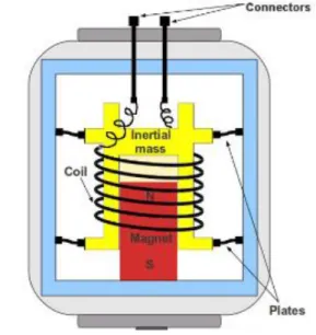
Seismic information has been procured through movement detecting geophone. Geophone is based on a proof mass suspended from a spring. The mechanical design of geophone as shown in Figure 1 below. A small permanent magnet is attached to its casing that provide a magnetic field in a cylindrical coil [10]. The cylindrical coil is suspended by light flat spring. For the geophone firmly fixed into the ground, the magnet takes after those ground movement inasmuch as the coil tries with remain stationary due to its inertia. The relative movement the middle of those coil and magnet has the ability to produce an electrical voltage [11, 12]. The signal captured by the geophone is then transferred to the recording instrumentation through a connecting cable where it is amplified and stored. Voltmeter is used to record the voltage is proportional to the velocity where the ground is moving [13, 14]. The orientations of the coil inside the geophone casing either it is in vertical movements or horizontal movements are measured[15].
Figure 1 Mechanical design of geophone
5
2.1.1 ELECTROMAGNETIC PRINCIPLE
The system uses electromagnetic induction principle which is according to Faraday’s law:
𝑣 ∝ 𝑑𝑥
𝑑𝑡 (2.1) where v represents voltage and x is the displacement of the magnet relative to the coil, while voltage is converted from the velocity of the proof mass inside the geophone element. The position of the proof mass is not affected by the system where the two positions rating the movement. Hence, the information recorded is the magnet velocity for the coil times with the sensitivity constant in Volts per velocity (Volt/m/s).
Geophones are based on a proof mass suspended from a spring that governs by the“forced simple harmonic oscillator equation:”
𝜕
2𝑥
𝜕𝑡2 + 2λω0∂x
∂t+ ω02x =∂
2u
∂t2 (2.2) where u is the ground displacement as well as the case displacement in permanent position, λ is the damping ratio and 𝜔0represents the resonant frequency.
Furthermore, geophone generates an analog voltage (𝑣𝐺) which is equal to the sensitivity multiply with the proof mass velocity, therefore;
𝑣𝐺 = 𝑆𝐺𝜕𝑥
𝜕𝑡 (2.3) 𝑆𝐺 represents the sensitivity constant of the geophone (in V·s/m). The strength of magnetic field as well as the number of loops in the coil represents the sensitivity of the geophone.
Next, it is proven that proof mass is related to ground motion (based on Equation 2.2), the analog output voltage expression can be obtained in terms of ground motion;
𝜔 = 1
𝐹 (2.4) The partial differential from Equation (2.2) is solved by replacing time derivatives with jω through the Fourier Transform method, where 𝑗 = √−1 . The equation is then transformed into the frequency domain;
−𝜔2𝑋 + 2𝑗𝜆𝜔0𝜔𝑋 + 𝜔02𝑋 = −𝜔2𝑈 (2.5)
6
X and U are frequency-domain representations of x and u. The continuation gives
𝑋(𝜔) = −𝜔2
−𝜔2+2𝑗𝜆𝜔0𝜔+𝜔02𝑈(𝜔) (2.6)
In engineering texts,
𝑋 = 𝑈 (𝜔
𝜔0)2𝐹 (2.7)
where
𝐹 = −1
− 𝜔2 𝜔02+2𝑗𝜆𝜔
𝜔0 +1
(2.8)
The expression above is for proving mass displacement (X) is related to the ground displacement (U). Based on the Equation (2.7), the resonance (𝜔0) and damping (λ) of the sensor are obtained from the displacement of proof mass from the ground.
The analog signal is generated according to proof mass velocity (∂x/∂t). The starting point can be taken from Equation (2.6) to consider all other domains of proof mass motion and ground motion, using the provision that ∂/∂t may be replaced with jω. As the result, Equation (2.6) can be considered as a general solution, jω can be modified depending on the specific domains required.
7
2.2 GEOPHONE CIRCUIT
Geophone is considered as a passive instrument which has to be suitably damped. As a ground movement detecting sensor, the initial ground movement will triggered a slow decreasing oscillations which has to be suppressed [16]. In normal geological experiments using geophones, the only electronic component or circuit used is by connect the damping resistor, Rd, parallel with the induction coil as shown in the Figure 2 below. The sum of the value of the damping resistor and the resistance of the moving coil, Rcoil, is the total damping resistance of the sensor.
Figure 2 Geophone damping resistor circuit
According to [16], a low damping resistor is good for the system by increasing the range of decreasing amplitude signal. However, the minimum value of Rd is 0Ω leaving just Rcoil alone, which is impossible to use with negative value of resistor in a real life. Figure 3 below is the configuration of the real life geophone connected with the damping resistor for the geological experiment.
Figure 3 Geophone element connected with the damping resistor
8
2.3 LOW LEVEL FREQUENCY DETECTION
Geophone is not suitable sensor to be used in all ground detection movement. As the geophone operates below its resonance frequencies level, the noise increases [14]. The high presence of noises makes the geophone as a poor sensor for applications that are using low frequency level detection. For seismic exploration in detecting earthquake, a precise, high sensitivity and low noise level is required to obtain an accurate data [14, 17].
According to [17, 18], the performance of the sensor is limited to the limit below resonant frequency of 10Hz according to the fundamental resonance of the inertial mass.
Figure 4 Sensitivity curve of geophone operated in open circuit condition and closed system with feedback loop (addition damping resistor)
Referring to [19], the sensitivity of the system which is the particle velocity that corresponds to one bit of the ADC output;
Sensitivity System = Sensitivity AMP h
Sensitivity GEOPHONE (2.8)
9
2.4 AMPLIFIER AND FILTER
Without modifying a geophone, the only term of “geophone” is referred to mean a vertical, horizontal or multicomponent geophone [20]. Mostly, the external apparatus is invented for the future use for example an invention employs a preamplifier to amplify the geophone signal and connected filter. The output of the signal is can be measured using level detector such as an oscilloscope. By amplifying the response of the input signal, the output is enhanced into a readable and measurable data to be used in seismic exploration [21].
According to [22], there are two options to extend the range of frequencies. First is through using low frequency sensor. However, it can be really costly for a large scale surveys.
Second option is through processing method to recover a low frequency signals for instance by inverse filtering or deconvolution. Inverse filter is a well-known technique to compensate low frequency components of geophone data [23]. The main of this technique is outlining the inverse filter, which is the frequency response reversal of the instruments.
Typically the frequency response bend is referring to the instrument manufactory, yet those reaction bends just incorporate a little measure of the low frequencies underneath the resonant frequency under the condition free of the self-noise.
The frequency range of the inverse filter, is determined by the two corner frequencies because a noisy artifacts would be produced if the design is an unlimited inverse filter.
There are low corner frequency and high corner frequency that determined the range of the inverse filter.“In this study both the inverse filter and the lowest retrievable frequency are estimated through the analysis of the power spectral density ratio (PSDR) based on co-deployed geophone and low-frequency digital phone data. The estimated lowest retrievable frequency for a field data acquired using 10-Hz geophones is 2 Hz. The stack section shows a stable recovery of low-frequency signals and enhancement of SNR using the PSDR method [22].”
10
CHAPTER 3
METHODOLOGY 3.1 PROJECT FLOW CHART
Start
Design damping resistance
Setting response
Setting offset
Setting frequency (1Hz-30Hz)
Output measurement at shunt resistor (1000 Ω)
Critical damp output (voltage)
Amplifier design
Circuit design
Amplified response
Amplitude increased
Filter design
Low pass filter design
Filtered response
Noise
End No
Yes
Yes No Yes
No
11
3.2 PROJECT INITIALIZATION
The choices of tools and equipment are selected after the literature review has been studied. In this project, redesigning damping resistor of the geophone is the aim of the project. The following studies has been done before the experiment:
1 Component geophone studies:
A single component geophone (1C) is use in conducting the experiment.
The output voltage is recorded according to the variation range of frequencies. The geophone is dipped into the ground in vertical position in order to get wave reflection effectively [24, 25].
Circuitry design:
An amplifier circuit and a filter circuit have to be designed in order to test the results when the geophone is connected with an oscilloscope. The design of the circuit should consider the gain of the amplifier circuit and the type of filter should be used in the design for the stability of the overall circuit. The gain of amplifier is set to set the level of amplification of the geophone response in voltage. In this project, the gain is set almost the same as the actual output response voltage level of the geophone without connected with the damping resistor.
Comparison between geophone connected with damping resistor with amplifier and filter circuit:
At the end of the experiment conducted, the comparison of results between geophone sensitivity is measured with damping resistor with geophone connected with amplifier and filter circuit with an oscilloscope connected to analysis the output waveform. The adjustment should be made to the circuit if the result is not achieved. The adjustment of the circuit is referring to the gain of the amplifier circuit as well as the low pass filter.
12
3.3 PROJECT DEVELOPMENT
In this stage, the focus is the amplifier and filter circuit design. Procedures for conducting the project are:
Experimental block diagram
A study regarding the block diagram to conduct the experiment is set and the simulation of the expected outcome should be obtained. Figure 5 shows a geophone is connected to the oscilloscope through the damping resistor, amplifier and filter circuit.
Figure 5 Experimental block diagram
Figure 6 Experimental apparatus and connections
13
Amplifier and filter circuit design
There a lot of researches and studies regarding the amplifier filter circuit design.
The amplifier is designed to amplify the current output response in terms of voltage based on the experiment previously which is using damping resistor.
However, the amplification process will invite external disturbances [26].
Therefore, the criteria of the filter circuit design should be considered in terms of its operations and the functions to improve the sensitivity of the geophone when it is connected with the oscilloscope. The filter circuit must be able to eliminate the noise above the cutoff frequency of the response.
3.3 TOOLS AND EQUIPMENT
Tools and equipment for conducting the experiment as follows:
Geophones element (SM-24)
Function generator (Model: Instek)
Oscilloscope (Model: Tektonix)
Damping resistor (1000Ω)
Amplifier circuit (Gain: 2.0 V/V ± 0.2 V/V)
Filter circuit (Low pass filter)
14
3.4 GANTT CHART AND MILESTONE
FYP 1 Week
Activities 1 2 3 4 5 6 7 8 9 10 11 12 13 14 Project topic
selection Problem Statement Objectives and Scope of studies Literature review Geophone Oscilloscope Design Amplifier review Resistivity review
Amplifier and Filter
Experiment design
15
FYP 2 Week
Activities 1 2 3 4 5 6 7 8 9 10 11 12 13 14 Prototype
Design
Amplifier circuit Filter circuit Lab testing Damping resistor
Amplifier circuit Filter circuit Amplifier &
filter circuit Report writing
symbol represents a Milestone
16
CHAPTER 4
RESULTS AND DISCUSSION
4.1 GEOPHONE EQUIVALENTS
According to [27], a geophone’s configuration to detect the movement of the earth by either placed onto the surface of the ground or by stuck into the ground using spike housing. The motions of the earth is exchanged to the geophone’s casing which the movement is related to the movement of coil inside the geophone. The current passing through the coil will be induced a magnetic field and the induction induced an emf.
The velocity from the casing and the result of the emf across the coil is related and can be computed from:
ῡ
𝑣
=
1𝐵𝜋𝑑𝑛 (4.1) where;
ῡ represents velocity to coil
B represents flux density of the magnet
v represents emf across the coil
d represents diameter of the coil
n represents number of turns of the coil
Figure 7 shows the geophone’s mechanical and electrical analogous circuit.“The geophone case, its spring and its mass behave in a similar way to the suspended rubber band and weight system. In addition, the geophone has a coil attached to the mass with an air gap of the magnetic circuit.”As the vertical force of ground motion is applied and the motion detected by the case, the significant mass moves in the direction of the applied force,“while the mass to which the coil is attached tends to resist the motion.”Figure 8
17
shows the electrical equivalent circuit of the geophone to find the energy transfer to the load with the value of components used are based on SM-24 specification and data sheet in APPENDIX 1 and APPENDIX 2.
Figure 7 Geophone’s mechanical and electrical analogous circuit
Figure 8 Geophone’s electrical equivalent circuit
Damping resistance
18
Ohms (4.2) Henries (4.3)
Farads (4.4) Where the acronym representations are
𝑅𝑒𝑞 is internal resistance equivalent 𝐶𝑒𝑞 is internal capacitance equivalent 𝐿𝑒𝑞 is internal inductance equivalent 𝐵 is open-circuit damping
𝐾 is spring stiffness 𝑀 is mass
𝐺 is sensitivity
Figure 9 Output gain from damping resistance geophone
19
4.2 CIRCUITRY DESIGN
Based on the circuitry design shown in Figure 10, there are parameters to be set in order to conduct the experiment of circuit prototype.
Figure 10 Amplifier and low pass filter design
This circuit consists of two circuits which are amplifier and low pass filter circuit. The input supply to the circuit is in terms of ground motion from the geophone. The amplifier circuit is made up of an operational amplifier (op-amp). The gain of the amplifier is varied by changing the value of R2 and to determine the gain value (A) of the amplifier as refer to the Equation 4.5 below.
𝐴 =𝑅1+𝑅2
𝑅1 (4.5) The filter circuit design is low pass filter where it is functioning to filter out noise when the circuit operating in low level frequency. It consists of a unit if resistor and capacitor to cut off the noise above the cutoff frequency and smooth the graph.
Low pass filter
20
4.3 EXPERIMENTAL RESULT
Table 1 Output response geophone SM-24 and 1000 Ohm damping resistor values Frequency SM-24 (mV) 1000 Ohm (mV)
1 Hz 55.26 32.27
2 Hz 65.27 40.76
3 Hz 77.64 53.31
4 Hz 86.84 57.16
5 Hz 92.92 68.08
6 Hz 96.34 73.45
7 Hz 100.95 78.20
8 Hz 102.21 82.47
9 Hz 128.82 86.61
10 Hz 135.77 87.12
20 Hz 156.81 102.38
30 Hz 157.67 102.68
Figure 11 Output graph based on Table 1
0.00 20.00 40.00 60.00 80.00 100.00 120.00 140.00 160.00 180.00
1 Hz 2 Hz 3 Hz 4 Hz 5 Hz 6 Hz 7 Hz 8 Hz 9 Hz 10 Hz 20 Hz 30 Hz
Amplitude (mV)
Frequency
Output response geophone SM-24 and 1000 Ohm damping resistor values
SM-24 (mV) 1000 Ohm (mV)
21
Experiment was conducted based on the circuit diagram as shown in Figure 10. The experiment was setup using two units of geophones in a container filled with soil and apparatuses as shown in a Figure 6. Frequencies vary from 1Hz to 30 Hz.
Based on the experimental results shown in Table 1 and Figure 11, geophone in opened circuit condition with no load resistor added. 1Hz frequency gives high starting amplitude of 55.26mV. This response is an overshoot output where it is one of the disadvantages of this geophone which it makes data processing more difficult [7]. Other than that, the large initial amplitude is due to the vibration of ground movement at low frequency [28]. Based on the graph on Figure 11, it shows a diverge of the output response between output response of original SM-24 geophone and geophone with damping resistor at frequency 8 Hz to 30 Hz. The output response of the original SM-24 geophone is highly accelerated and unstable while with addition of damping resistor, the output response is increasing accordingly as the frequency increases.
SM-24 geophone is connected to the damping resistor of 1000 Ohm value. Damping resistors or shunt resistors give more stable output but it lower the amplitude of voltage detected in low level frequency [16]. The damping resistor control the movable components inside the geophone to make the curve smooth [4]. Based on the experimental result, 1000 Ohm shunt resistor resulting more smooth and stable graph compared to the original output response of SM-24 geophone in frequency 8 Hz to 30 Hz. As cited by [16]
earlier, lowering the amplitude of voltage detected in connecting shunt resistor is proved by conducting the experiment and the results as shown in Table 1 and Figure 11.
22
Table 2 Output response of SM-24 geophone connected with 1000 Ohm damping resistor and three different amplifiers with different gain
Figure 12 Output graph based on Table 2 Frequency
SM-24 (mV)
1000 Ohm (mV)
Amplifier 1 (mV)
Amplifier 2 (mV)
Amplifier 3 (mV)
1 Hz 55.26 32.27 43.53 46.71 54.75
2 Hz 65.27 40.76 64.19 60.78 66.62
3 Hz 77.64 53.31 84.79 70.16 70.94
4 Hz 86.84 57.16 84.47 78.12 79.32
5 Hz 92.92 68.08 95.05 91.37 87.01
6 Hz 96.34 73.45 106.95 96.56 97.94
7 Hz 100.95 78.20 114.94 111.82 116.71
8 Hz 102.21 82.47 126.41 116.31 121.38
9 Hz 128.82 86.61 125.79 122.83 126.53
10 Hz 135.77 87.12 153.53 140.16 140.97
20 Hz 156.81 102.38 216.63 182.59 165.27
30 Hz 157.67 102.68 155.54 146.56 148.96
0.00 50.00 100.00 150.00 200.00 250.00
1 Hz 2 Hz 3 Hz 4 Hz 5 Hz 6 Hz 7 Hz 8 Hz 9 Hz 10 Hz 20 Hz 30 Hz
Amplitude (mV)
Frequency
Output response of SM-24 geophone connected with 1000 Ohm damping resistor and three different amplifiers with different
gain
SM-24 (mV) 1000 Ohm (mV) Amplifier 1 (mV) Amplifier 2 (mV) Amplifier 3 (mV)
23
Referring to the result shown in Table 2 and Figure 12, 1000 Ohm shunt resistor is proceed in conducting the second stage of the experiment. The 1000 Ohm shunt resistor is connected to three different amplifiers with different gain value. Three different circuits of amplifier were tested in order to obtain stable point. Therefore, value of components of the amplifier circuit which is the value of resistor (R1) was adjusted to give an output from the geophone with the gain of the amplifier sets to 2 V/V ± 0.2 V/V. Table 2 and Figure 12 show the result of geophone response when connected to Amplifier 1, Amplifier 2 and Amplifier 3 circuits with the gain rated as 2 V/V, 1.8 V/V and 2.2 V/V respectively.
From the graph, amplifier amplify the geophone response in terms of its voltage amplitude when the geophone operate at lower than its natural frequency response. As the amplifier amplify the output response of the geophone connected to the 1000 Ohm shunt resistor Amplifier 1 circuit recorded unstable frequency from 3 Hz to 9 Hz while Amplifier 2 circuit is unstable from 5Hz to 7 Hz. Amplifier 3 recorded the most unstable output in amplifying the geophone response with 1000 Ohm damping resistor from 2 Hz to 30 Hz frequency. In frequency 8 Hz to 30 Hz, the output response amplified as expected.
However, at 20 Hz, all three amplifier circuits experience the high peak amplitude. The variations of peak amplitude are according to the gain of the amplifier. As the gain increases, the lower the sharp peak amplitude. The strong and sharp peak of the graph shows the resonant frequency for the geophone when it is connected to the amplifier circuit.
24
Figure 13 Output graph based on Table 3
Table 3 Output response SM-24 geophone connected with 1000 Ohm damping resistor, three different amplifiers and low pass filter
Frequ- ency
SM-24 (mV)
1000 Ohm (mV)
Amplifie r 1 (mV)
Amplifier 2 (mV)
Amplifier 3 (mV)
Filter 1 (mV)
Filter 2 (mV)
Filter 3 (mV)
1 Hz 55.26 32.27 43.53 46.71 54.75 41.17 43.62 51.65
2 Hz 65.27 40.76 64.19 60.78 66.62 57.35 55.85 61.02
3 Hz 77.64 53.31 84.79 70.16 70.94 72.50 65.42 68.76
4 Hz 86.84 57.16 84.47 78.12 79.32 80.94 75.37 76.46
5 Hz 92.92 68.08 95.05 91.37 87.01 93.52 91.37 87.01
6 Hz 96.34 73.45 106.95 96.56 97.94 98.78 94.89 95.78 7 Hz 100.95 78.20 114.94 111.82 116.71 100.94 97.88 103.34 8 Hz 102.21 82.47 126.41 116.31 121.38 112.57 109.53 114.68 9 Hz 128.82 86.61 125.79 122.83 126.53 120.39 116.85 121.64 10 Hz 135.77 87.12 153.53 140.16 140.97 131.41 125.87 128.44 20 Hz 156.81 102.38 216.63 182.59 165.27 149.67 140.98 144.39 30 Hz 157.67 102.68 155.54 146.56 148.96 142.50 136.97 140.62
0.00 20.00 40.00 60.00 80.00 100.00 120.00 140.00 160.00 180.00
1 Hz 2 Hz 3 Hz 4 Hz 5 Hz 6 Hz 7 Hz 8 Hz 9 Hz 10 Hz 20 Hz 30 Hz
Amplitude (mV)
Frequency
Output response SM-24 geophone connected with 1000 Ohm damping resistor, three different amplifiers and low pass filter
SM-24 (mV) 1000 Ohm (mV) filter 1 (mV) filter 2 (mV) filter 3 (mV)
25
Table 3 and Figure 13 show the output response of the geophone when connected with an amplifier circuit together with a filter added to the circuit. In order to overcome the strong peak graph output, a low pass filter is used [29]. The function of the low pass filter is to eliminate frequency above the cutoff frequency and make the graph smoother without having a sharp peak [30]. The RC low pass filter is designed to filter and response.
The output response of the geophone connected with shunt resistor, amplifier as well as filter show an improvement. The main objective is to reduce the high peak output at 20 Hz frequency. The comparison can be made before and after the filter is added to the amplifier circuit. Amplifier 1 reduces the peak resonant by 31% while Amplifier 2 and Amplifier 3 reduced by 23 % and 13% respectively. At frequency 8 Hz to 30 Hz, the output responses are filtered and become more stable. The responses show no changes of diverge nor converge which all responses recorded the same output pattern. Stability output response shows Amplifier 1 circuit recorded unstable frequency from 6 Hz to 8 Hz while Amplifier 2 circuit is unstable from 5 Hz to 7 Hz. Amplifier 3 recorded the best output in amplifying the geophone response with 1000 Ohm damping resistor.
26
Table 4 Final output response selected for SM-24 geophone connected with 1000 Ohm damping resistor, amplifier and low pass filter
Frequency
SM-24 (mV)
1000 Ohm (mV)
Amp 3 (mV)
Filter 3 (m)
1 Hz 55.26 32.27 54.75 51.65
2 Hz 65.27 40.76 66.62 61.02
3 Hz 77.64 53.31 70.94 68.76
4 Hz 86.84 57.16 79.32 76.46
5 Hz 92.92 68.08 87.01 87.01
6 Hz 96.34 73.45 97.94 95.78
7 Hz 100.95 78.20 116.71 103.34
8 Hz 102.21 82.47 121.38 114.68
9 Hz 128.82 86.61 126.53 121.64
10 Hz 135.77 87.12 140.97 128.44
20 Hz 156.81 102.38 165.27 144.39
30 Hz 157.67 102.68 148.96 140.62
Figure 14 Output graph based on Table 4
0 20 40 60 80 100 120 140 160 180
1 Hz 2 Hz 3 Hz 4 Hz 5 Hz 6 Hz 7 Hz 8 Hz 9 Hz 10 Hz 20 Hz 30 Hz
Amplitude (mV)
Frequency
Final output response selected for SM-24 geophone connected with 1000 Ohm damping resistor, amplifier and
low pass filter
SM-24 1000 Ohm (mV) Amplifier 3 Filter 3
27
After all three stages of experimental conducted with SM-24 geophone, the selected value of damping resistor as well as the amplifier and filter circuit are chosen. The comparison of changes of the geophone response can be seen from Figure 14. The unstable output response for SM-24 geophone from 8 Hz to 30 Hz are reduced by adding a damping resistor with 1000 Ohm value. The output from damping resistor showing a high damping output and the response is smoother. Hence it shows that the SM-24 geophone can be operated in low frequency range of 1 Hz to 30 Hz. Next, in order to increase the amplitude as much as same as the original SM-24 response, an amplifier circuit is added. Even though the output response recorded is unstable from 2 Hz to 30 Hz frequency, however, when the filter circuit is added, the output response become smoother. The low pass filter selected to cancel the undesired response resulting a better quality of output response. The high peak amplitude at 20 Hz frequency from amplifier circuit is reduced by 13%.
Therefore, SM-24 geophone can be operated in low frequency of 1 Hz to 30 Hz.
28
CHAPTER 5
CONCLUSION AND RECOMMENDATION
5.1 CONCLUSION
In conclusion, a geophone’s performance can be improved by designing the external circuit of amplifier and filter circuits. The cost of buying an equipment to enhance the performance of this seismic sensor is expensive. Thus, theoretically, a simple low cost amplifier and filter prototype can be designed in order to get the better performance for the geophone as a seismic sensor to detect lower frequencies than its resonant.
An experimental study has been performed in the lab provided to proof the concept of amplifier and filter when geophone is connected to an oscilloscope. The range of frequency set for the experiment is between 1 Hz to 30Hz. The results show an improvement on the geophone performance to operate at lower frequency below its resonant. Based on the experiment, SM-24 geophone alone gives higher starting amplitude and the amplitude is varying proportional with the frequency. However, the output response is undesirable because it acts aggressively in open circuit due to the aluminum coil acting as a single coil and shorted the circuit causing a large current flowing in the coil.
The geophone is connected to the damping resistor of 1000Ω to suppress and control the movable component inside the geophone. The response of the geophone is recorded more stable however it lower the amplitude voltage level. Next, the geophone then connected to the amplifier circuit with voltage gain is set to 2 V/V in order to amplify the response to the higher level which is as the same as the original voltage amplitude level of the geophone. Three different amplifier circuits with plus minus 0.2 V/V gain are designed and connected to the geophone to obtain almost accurate geophone original voltage amplitude level. However, the amplifier circuit still can be adjusted to have higher gain to get higher amplitude output response from the device.
29
Based on the amplifier circuit designed, the amplifier manages to operate from 8Hz to 20Hz if more than, the amplitude is decreasing as the frequency increasing. This situation occurs because the amplifier designed has reached its resonant frequency.
Other than that, the sharp peak resonant frequency can be detected due to the low damping. Hence, a low pass filter is added to the amplifier circuit in order to eliminate frequency above the cutoff frequency resulting a smoother graph without any sharp peak output response.
Next, from the graph of the output response of the amplifiers and geophone, the most stable frequency response is recorded at 6Hz and 8Hz. Further experiment of geophone connected with shunt resistor, amplifier and filter circuit is required to obtain the optimum result of performance of the geophone in operating at lower frequency. Last but not least, further studies should be taken in order to develop the implementation of the design in real seismic explorations.
5.2 RECOMMENDATION
SM-24 geophone can obtain 60% of damping response using damping resistance value of 1339Ω according to APPENDIX 1. Some changes can be done to the circuit which probably give benefits in detecting lower frequency of the device. The changes can be done by replacing the components used for the circuit as well as increasing the gain of the amplifier or by adding filter stages to improve filtering process of the response. In addition, the amplifier and filter circuit can be printed on printed circuit board to get better stability components connections from loose as well as to make it more portable for the testing.
viii
REFERENCES
[1] Y. C. a. D. Qiao, Design of Digital Geophone System Based on FPGA, 2015.
[2] W. Ding, Development of Capasitive Position Sensing Geophone for Microtremor System, 2013.
[3] M. E. Everett, "Near-Surface Applied Geophysics," 2013.
[4] W. O. McNeel, Geophone Having Electromagnetic Damping Means, 1977.
[5] J. Dams, Magnetic Innovation in Velocity Sensing Low Frequency with Passive.
[6] A. Pap, Criteria for the selection of geophone parameters, hookups, phone spacing and low cut instrument filters, 1984.
[7] P. E. Stephen K. Chu, Jack Howell and Jeff Malloy, The feasibility and value of low-frequency data collected using colocated 2-Hz and 10-Hz geophones, 2013.
[8] G. B. Bowden, Calibration of Geophone Microseismic Sensors, 2003.
[9] T. L. L. Rune Brincker, Palle Andersen and Carlos Ventura, "Improving the Classical Geophone."
[10] J. M. Reynolds, "An Introduction to Applied and Environmental Geophysics,"
2011.
[11] S. K. Upadhyay, "Seismic Reflection Processing," 2004.
[12] B. Holden, Low Frequency Improvements to Commercial geophones, 2014.
[13] T. Boyd, Geophones.
[14] S. M. Tom Kenny, Tom Pike, Tom VanZandt and Aaron Barzilai, An affordable broadband seismometer : The capacitive geophone.
[15] P. J. G. a. D. M. George, "Environmental Applications of Geophysical Surveying Techniques," 2013.
[16] B. Ulmann, Overdamping geophones using negative impedances, 2005.
[17] P. C.-F. C. Collette, S. Janssens, K. Artoos, M. Guinchard, C. Hauviller, Review of sensors for low frequency seismic vibration measurement, 2011.
[18] L. F.-R. Christophe Collette, Mihaita Horodinca, Prototype of a small low noise absolute displacement sensor, 2013.
ix
[19] G. K. a. K. Yegin, Hardware Design of Seismic Sensors in Wireless Sensor Network, 2013.
[20] E. D. Bednar, Geophone Checker, 1987.
[21] L. H. Francis G. Blake, Calif,, Amplifier Circuit Having Linear and Non-linear Amplification Ranges, 1952.
[22] Z. Z. a. H.-w. Z. Yimeng Zhang, Estimating and recovering the low frequency signals in geophone data.
[23] J. H. a. G. Alguacil, "Instrumentation in Earthquake Seismology," 2004.
[24] Z. S. Gang Tian, Shixue Dong and Zhejiang Wang, "Geophone Coupling Match and Attenuation Compensation in Near Surface Seismic Exploration."
[25] C. E. Krohn, Geophone Ground Coupling, 1984.
[26] J. d. R. X.Roset, A.Manuel and R. Palomera-Garcia, Contribution to Model Characterization of Geophone Sensor, 2004.
[27] A. Stark, "Seismic Methods & Applications," 1946.
[28] M. S. Hons, Seismic sensing: comparison of geophone and accelerometers using laboratory and field data, 2008.
[29] J. H. a. G. Alguacil, "Instrumentation in Earthquake Seismology," 2006.
[30] E. Ramsden, An Introduction to Analog Filter, 2001.
x
APPENDIX 1
Physical specification of geophone element (SM-24)
xi
APPENDIX 2
SM 24 Electrical Parameter
Based on the geophone equivalent circuit shown in Figure 1 below, the parameters are find in order to construct and simulate the circuit.
Ohms (4.2)
Henries (4.3)
Farads (4.4) The constant geophone parameters can be obtained from Appendix 1.
Rc = 375 Ω Lc = 32mH M = 11g G = 28.8v/m/s fo = 10Hz
D = 0.25 (open damping) Calculated values:
Req = 2.40kΩ Leq = 19.1H Ceq = 13.5uF
Figure 1 Geophone electrical equivalent circuit