This study aims to improve the Dixon Coles model by implementing attack and defense parameters at the player level. In this context, a player's attack and defense parameter is calculated from player rating data coming from whoscored.com(n.d.). Using the Dixon Coles model (before and after adding the player's parameter), we predicted matches for the entire season, and the results of both models were compared.
A more accurate estimate will be obtained by considering the player's recent performance as an additional parameter. They calculated each player's rating for each game by taking into account every event recorded in the games. Each player's recent performance can be considered to build the model, as a player's performance can directly affect the team's performance.
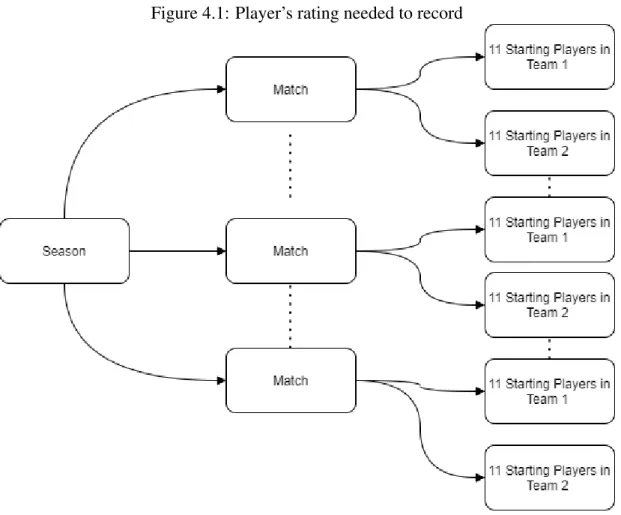
Therefore, it is essential to evaluate the football match from the team's perspective and the player's perspective. By taking the individual's rating from the previous match, we can assess the player's recent form and provide a more accurate prediction insight. Some data is needed, such as past score and player rating for each match.
We reconstruct two Dixon Coles models using R, one for the original model and another implements the player rating.
C HAPTER 2: L ITERATURE R EVIEW
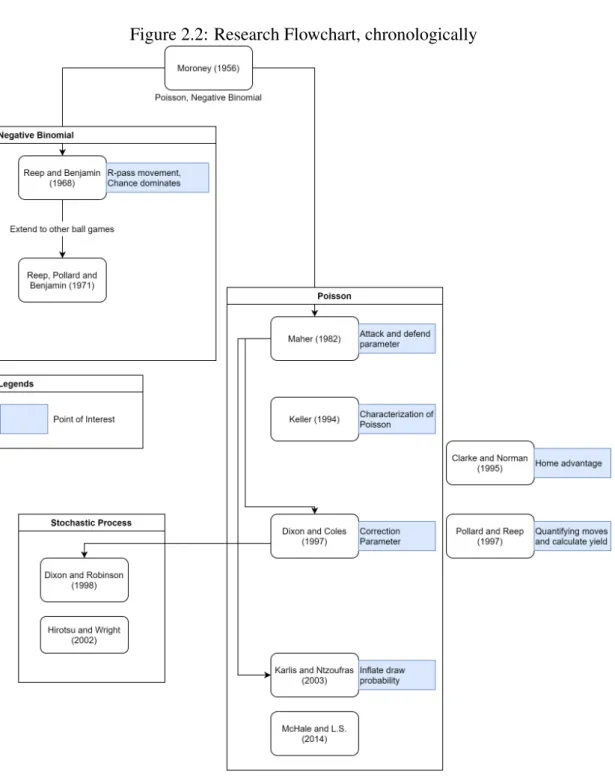
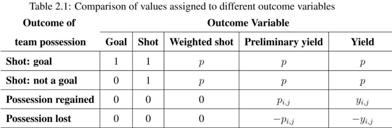
The probability p that an attack will result in a goal is small, but the number of times a team has possession during a game is large. If p is constant and attacks are independent, the number of goals will be Binomial, and in these circumstances the Poisson approximation will apply very well. The mean of this Poisson will vary depending on the team's quality, so if one considers the distribution of goals scored by all teams, one will have a Poisson distribution with variable means.
However, Maher's model has underestimated the number of goals with one and two goals scored and overestimated the number of ≥4 goals and 0 goals. Assume that the opponent with the highest score wins and that pn is Poisson distribution with meanλ, then for any distributionqn,. He has shown that the standard deviation of Expected Wins & Draws and Actual Wins & Draws is reasonably small in his work, indicating that the model fits the data.
Clarke (1995) made the point that home field advantage is different for each individual club and that the size of the advantage is linearly related to the distance between the two playing clubs. Please note that this benefit may not apply in 2020 due to the COVID-19 pandemic as most major leagues play with empty stadiums. Their research found that the model underestimates the probability for lower-scoring games, such as.
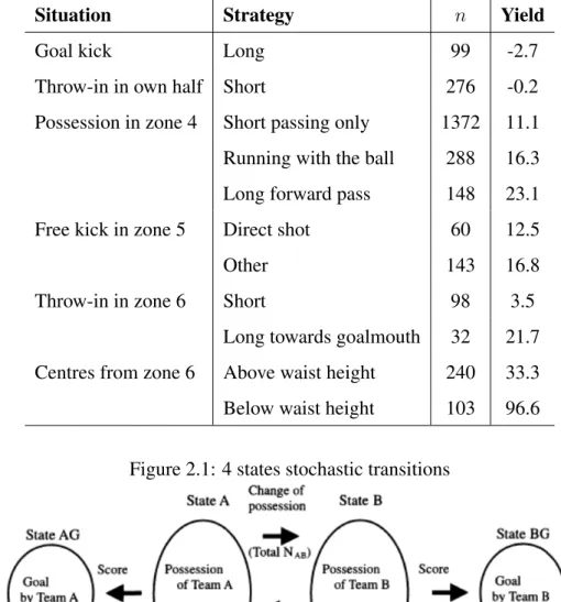
In the sense that the more recent assessment will have more influence compared to the previous assessment. Due to the nature of the birthing process, this model must calculate the probabilities of being in each state during 90 minutes of gameplay. Note that the negative yield indicates that the strategy would, on average, result in more goals conceded than scored.
Pollard (1997) did not involve any statistical distribution, but this has shown us that playing strategy can be quantified and we can apply this further in our research. In the negative binomial approach, C.Reep (1968) categorizes events that happen on the track, categorizes the events according to the number of passes that occurred, and the number of occurrences was used as the parameter for negative binomial. Dixon (1998) considers the time remaining in the game and the current score, treating the number of goals as interacting birth processes.
C HAPTER 3: P RELIMINARY R ESULT
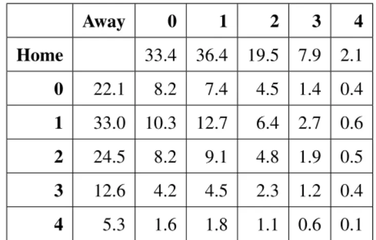
Having estimated the parameters, we predict the score matrix for a match, Arsenal vs. We can further see that the probability of the winning result for this match is Arsenal Win 0.4253858.
C HAPTER 4: R ESULTS AND D ISCUSSION
Referring to Figure 4.7, the first table in the figure shows the league we have. We have the start time of the match, the teams playing in the match and the final result. When we navigate further, by clicking on the Detail button in each row, we can see the details in the match.
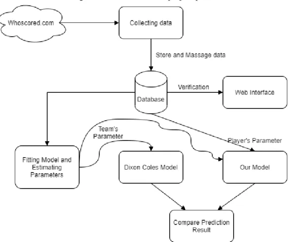
As shown in Figure 4.8, the data displayed in our user interface is the same as the data displayed inwhoscored.com (n.d.). From the data we collected from whoscored.com (n.d) we will use match date, playing teams, final score and the list of player ratings. After getting the data ready in the database, we will go through the player's rating and calculate our player's attack and defense ability parameters.
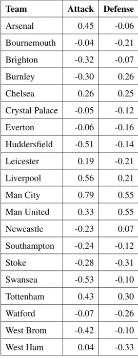
So, in our model, their assessment will be taken into account in the calculation of both attack and defense parameters. Moving forward from here, we can calculate the player's offense and defense parameters by averaging the players' rating on the offensive and defensive ends. We modify the above model by implementing four new parameters, which we obtained from player rating, Home Attack (HA), Home Defense (HD), Away Attack (AA) and Away Defense (AD) into the model Dixon-Coles.
Using the α, β, γ, and ρ value discussed in chapter 3, and HA, HD, AA, AD value discussed earlier in this chapter, we get the following values, comparison between Dixon -Coles model and our Dixon-Coles with player rating. Dixon-Coles Model predicted Southampton's win at 42.6767%, while our improved model predicted Southampton's win at 84.95%. To perform this test, we first read all 380 matches for the 18/19 season from CSV, along with the participating team's name and player rating parameter (for the steps to obtain player rating parameter, refer to Figure 4.11).
For each match, we run a Dixon-Coles model and a Dixon-Coles model with player rating. A positive difference value indicating that our model predicts better, while a negative difference value means that the original Dixon-Coles model does a better job of forecasting. The Dixon-Coles model predicted a Southampton win probability of 15.24%, while our model predicts Southampton to win at 82.57%, a difference of 67.33%.
Dixon-Coles Model predicted that the away team wins at 61.94%, while our model predicts that the away team wins at only 4.86%. Among the 145 matches that we predict better than Dixon-Coles model, we predict on average 21.05% better.
C HAPTER 5: C ONCLUSIONS AND
R ECOMMENDATIONS
In this case, if we take the average, the player rating will be 7.4, which is a better reflection of the player's skill. We imagine a scenario where a mediocre player gets a phenomenal performance in one of the past matches. Our current model will get this player's rating to be 5, and if we apply the suggestion in point #3, the player's rating will be 6.
In our current model, we take the player's rating into account, but we ignore the fact that the same team may not play with the same player line-up in the . The protagonist may be rested/injured, or the manager may decide to rotate the squad, making our player's rating parameter not so meaningful. For example, the team equipped the critical player with a high rating, let's say a 9 in the last game.
So logically, if we take the resting player into our model's consideration, we might predict wrongly. However, substitution is also part of the game, and often a good substitution strategy will turn the tide of the game. In such cases, consideration of the substitute player's rating will have a positive influence on our prediction.
We consider a scenario: Arsenal is ranked #2, played with Leeds United ranked #20, Arsenal gets a higher player rating overall. This often happens, especially when the league is in the last few weeks, when some of the teams have secured the places or reached their goals for the season. Winning or losing the last few matches does not affect their result, so players are not motivated in the game and may play casually.
On the opposite side, some teams may be fighting to avoid relegation or promotion in the last few games, so their desire to win is higher. We may be able to make some adjustments for these cases whether the team is motivated or not. The underlying distribution in the Dixon-Coles model is the Poisson distribution, so as long as the event is statistically independent and the rate of what happens is constant, we can have a lot of use for this Poisson distribution.
R EFERENCES