PDF BIBLIOGRAPHY

ALOS, EMILY JUNE C., BAT-OY, ELEONOR B. April 2008. Efficiency of Ratio and Regression Estimators in Estimating Strawberry Production. Benguet, State University, La Trinidad, Benguet.

Adviser: Marycel H. Toyhacao

ABSTRACT

The study was conducted to determine the efficiency of the estimates on strawberry production using ratio and regression estimators.

A total of 195 plots were selected as samples from the total population of 899 plots from the Sariling Sikap area at strawberry farm. The data were summarized, tabulated and analyzed. The total production and total number of plants per area were used as the variables in the estimation.

Being an unbiased estimator, the Simple Random Sampling has the least mean and total production of strawberry. Among the bias estimator, classical ratio estimator is the most precise among the three estimators used in estimating strawberry production with its least coefficient of variability.

Regression estimator is the most consistent estimator and it is considered the most efficient estimator among the estimator used in estimating the strawberry production.

Page

Bibliography ………. i

Abstract ………. i

Table of Contents ………..………. ii

INTRODUCTION ……….. 1

Background of the Study ……… 1

Objective of the Study ……… 3

Importance of the Study ……… 3

Scope and Delimitation ……… 4

REVIEW OF RELATED LITERATURE ……….. 5

THEORETICAL FRAMEWORK ……….. 11

Simple Random Sampling ………... 11

Classical Ratio Estimation ……… 13

Hartley-Ross ratio-type Estimation ……… 16

Regression Estimation ……… 20

Magnitude Efficiency ……… 24

Definition of Terms ……… 25

METHODOLOGY ……… 26

Respondents of the Study ………... 26

Data Gathering ………... 26

Data Analysis ……… 26

Consistency of the Estimates ……… 29

Precision of the Estimates ……… 30

Relative Efficiency of the Different Estimates ……… 31

SUMMARY, CONCLUSION AND RECOMMENDATION …….. 33

Summary ……… 33

Conclusion ……… 34

Recommendation ……… 34

LITERATURE CITED ……… 35

APPENDICES ……… 37

Appendix A. Application for Oral Defense ……… 37

Appendix B.The raw data of the strawberry production ………….. 38

Appendix C. Sample Computations ……….. 43

INTRODUCTION

Background of the Study

A sample survey may be considered as an absolute (enumeration) experiment whose main objective are to obtain estimators of parameters and to derive measures of precision of these estimators. In analytical surveys one of the objectives is to test hypothesis with the use of appropriate estimation procedures.

Thus, it is apparent that simple and sound estimation techniques must be developed to provide precise and accurate statistics whether such endeavors are of the absolute or analytical type or both. (Burton T. Onate & Julia Mercedes O.

Bader: 1990)

Estimation of the population mean and total sometimes based on a sample of response measurements y₁,y₂,….y_n are obtained by simple random sampling and stratified random sampling. William Mendenhall (1990) stated that measuring Y and one or more subsidiary variables are used to estimate the mean of the response Y. It is basic to the correlation and provides means for development of a prediction equation relating Y and X by the method of least square.

The basic concept in estimation procedure is to determine the unknown values of the parameters using the sample values. By doing so, many estimators can be utilized. Among of those are using ratio estimators and regression estimators. However, the correct approach can lead to better estimates, that is, less bias is obtained. Ratio estimators and regression estimators, as pointed by Onate

and Bader (1990), increased its precision or usually attained by observing an additional variable Zi, in addition to the original characteristics.

It is most effective when the relationship between the response y and the subsidiary variable x is linear through the origin and the variance of y is proportional to x.

In Regression estimation the technique is for incorporating information on a subsidiary variable, this is better if the relationship between the y’s and x’s is a straight line not through the origin. It works well when the plot of y and x reveals points by lying uniformly close to a straight line with unit slope.

Ratio estimation usually leads to biased estimators. Thus, a consideration for the magnitude of the bias should be observed. However, for a large sample size (n>30) and he (σx/μx) ≥10, the bias is negligible. Ratio estimators are unbiased when the relationship between y and x is linear through the origin. As mentioned, we can assume to draw sample from the population, and possibly estimate its average (strawberry production) from y, sample mean. Since there are underlying associations between the mentioned variables, the number of plants per plot can be multiplied from the production of strawberries per plot.

Objective of the Study

Specifically, the study was conducted to determine the efficiency of the estimates on the production of strawberries in Strawberry Farm, La Trinidad, Benguet using the ratio estimates and using regression estimates.

Importance of the Study

The researchers find the study important; it gives information to the concern individuals specially in estimating the production of strawberry in La Trinidad, Benguet using the ratio and regression estimators. Through this study, students would be aware that strawberry production can be estimated or it can be measured using statistical tools by studies and researchers.

The useful and relevant information acquired from the study will encourage future researchers to estimate strawberry production applying the choice of their analysis. This can help them to boost their ability in analyzing given data’s from the specific tools they will conduct.

Result of the study will provide the strawberry management knowledge if the ratio and regression estimators can be appropriately applied to the production of strawberries. This will make them aware on the specific materials needed for strawberry production.

This study will serve as a valuable reference to farmers that production of strawberry can be estimated through different estimation procedures. This will also be a basis on how many strawberries will be produced in one plot.

Finally, this study will be an instrument or a benchmark for other researchers who are planning to study on different estimation procedures.

Scope and Delimitation

The main focus of this study was to determine the efficiency of ratio and regression estimators in the production of strawberries in Strawberry Farm at La Trinidad, Benguet.

The data was gathered from the Strawberry Farm of La Trinidad, Benguet.

Specifically at the Sariling Sikap Area.

REVIEW OF LITERATURE

Ratio Estimation

The ratio estimation is a different way of estimating population total or mean that is useful in many problems. It involves the use of known population totals for auxiliary variables to improve the weighting from sample values to population estimates. It operates by comparing the survey sample estimate for an auxiliary variable with the known population total for the same variable on the frame. The ratio of the sample estimate of the auxiliary variable to its population total on the frame is used to adjust the sample estimate for the variable of interest.

Ratio method of estimation is frequently used in sample surveys to estimate the population mean of the variable under investigation. Several ratio- type estimates can be formed. All these estimates are unsatisfactory in the sense that they are biased. Hartley and Ross, who proposed an unbiased ratio-type estimator for uni-stage sampling designs, overcame this difficulty. In practice, however, we are generally faced with multi-stage sampling designs. This communication gives a generalized form of Hartley-Ross unbiased ratio-type estimator for multi-stage designs.

This method aims to obtain an increased precision by taking advantage of the correlation between Yi and Xi .It applies population knowledge of adjustment variable X_i to improve estimation of the population total should be known.

The ratio estimates can be used when X_i is done some other kind of supplementary variables. However, for successful application, the ratio Yi / Xi

should be relatively constant over the population and the population total should be known.

Lohr (1999) enumerated the uses of ratio estimation which include: ratio estimators is simply used to estimate a ratio; to estimate a population total but the population size N is unknown and to adjust estimates from the sample so as to reflect demographic totals.Often,it is used to adjust for no response.

Hsu and Kuo (2000) used the ratio estimation to estimate the recycled and the production values and employment opportunities induced by household waste recycling. Ratio estimation was used in their study because the true population size of recycling plant is unknown; and the audited amount of household waste recycling is known; and the audited amount and recycling amount are highly correlated.

Angel et.Al (2004) evaluated the impact of using ratio estimation in their study, as the estimate census of night dwelling was much closer to the actual value.

M.Gossop, J.Strang, P.Griffiths, B.Powis and C.Taylor presents an approach in estimating the prevalence of cocaine use, based upon a new ratio estimation technique. This method can be applied to random samples of overlapping populations for which no sampling frames exist. When the ratio

estimation method is applied to the two studysamples (drawn from populations of people using cocaine and people usingheroin) the ratio of cocaine users to heroin users (C/H) was 1.55, with a95% confidence interval of +/- 0.48. Such estimates should be applied with caution. However, if used with reference to national estimates of about 75,000 heroin users, application of the present estimate suggests that there may be about 116,000 cocaine users in the UK.

Myers and Thompson (1989) pioneered the concept of a generalized approach to estimating hedge ratios, pointing out that the model specification could have a large impact on the hedge ratio estimated. While a huge empirical literature exists on estimating hedge ratios, the literature lacks a formal treatment of model specification uncertainty. These researches accomplish the task by taking a Bayesian approach to hedge ratio estimation, where specification uncertainty is explicitly modeled. Specifically, a Bayesian approach to hedge ratio estimation that integrates over model specification is uncertain; it yields an optimal hedge ratio estimator that is robust to possible model specification because it is an average across a set of hedge ratios conditional on different models. Model specifications vary by exogenous variables (such as exports, stocks, and interest rates) and lag lengths. The methodology is applied to data on corn and soybeans and results showed potential benefits and insights from such approach.

Damoslog and Tomin (2007) considered the Classical Ratio Estimation as a precise and efficient estimator because it has the lowest coefficient of variation and 15% higher relative efficiency than simple random sampling. They also cited that classical ratio estimator has the least estimated bias and is a consistent estimator with its narrow 95 % confidence interval

.

Regression Estimation

Regression estimation aims to find a relationship between a dependent variable and set of independent variable (Kweon and Kocelman, 2004).

In a study conducted by Wei Chen et.Al (2005), linear regression was used to evaluate the parameters with the least squares estimation to estimate an original model for daily shopping with the consideration of individual influence the estimation was verified to be straight forward and efficient.

Myall (2000) noted a known feature of regression estimation, that is, some data will generate negative and weights, which leads to having a download effect on aggregate estimates.

Valliant (2002) used the general regression estimator to construct variance estimators that are approximately model-unbiased in single estimates.

Barrios (1995) explored the used of various small area estimators for various socio-economic indicators. Regression estimation was noted to be reasonable use.

Watson (1937) from Cochran’s Citation (1977) illustrated an example of a general situation in which regression estimates are helpful. Watson used a regression on the leaf area and leaf weight to estimate the average area of the leaves on a plant. The procedure was to weight all the leaves of the plant. The area and the weight of each leaf were determined from the small sample of leaves.

The sample area was then adjusted by means of the regression on leaf weight means of the regression on leaf weight.

Usha Rani (2001) used the regression model Y=k (LxP) where Y = fruit surface area in Chili (capsicum annuum L.)Fruit, D= diameters of the fruit and k is the regression coefficient. She found the values of k=1.6827.Thus, one can estimate the fruit diameter x 1.6827.

Palaniswamy (1990) reported that the linear regression model can be employed in the prediction of grain yield per plot in rice and consequently for crop estimation.

Lih-Yuan Deng and RAJ S. Chhikara (1990) cited that in a classroom setting students often find the concept of super population and the assumption of a model somewhat artificial when one needs to estimate the mean of a finite population. They introduce the concept of a finite population decomposition based on a regression fit to the population values and then discuss the bias and variance of each estimator from the sampling design viewpoint. It shows by fitting a regression line of y and x to the finite population, that the leading term of

the bias of yˆ is accounted for it on terms of the intercept of the regression line. _R On the other hand, using quadratic regression fit, describe the leading term of the bias of yˆ in terms of the coefficient of the quadratic term. Moreover, the sign of _ir intercept in the fitted regression fit would be indicative of an over-or underestimation of Y by yˆ or _R yˆ ,respectively. They hope that this will add to _ir the understanding of the sampling properties of yˆ and _R yˆ without having to _ir assume the super population structure.

Dorfman, J.H and Sanders, D.R (2004) cited that regression and regression-related procedures have become common in survey estimation. It reviews the basic properties of regression estimators, discuss implementation of regression estimation, and investigate variance estimation for regression estimators. The role of models in constructing regression estimators and the use of regression in non-response adjustment are also explored.

A class of ratio and regression type estimators is given such that the estimators are unbiased for random sampling, without replacement, from a finite population. Nonnegative, unbiased estimators of estimator variance are provided for a subclass. Similar results are given for the case of generalized procedures of sampling without replacement. Efficiency is compared with comparable estimation sample selection methods for this case (Rand Corp Santa Monica Calif).

THEORETICAL FRAMEWORK

Simple Random Sampling (SRS)

Simple random sampling is a method of selecting n units out of the N population elements such that every ⎟

⎠

⎜ ⎞

⎝

⎛ n

N distinct sample has an equal chance of

being selected. (Beligan et al., 2004)

Yn is the unbiased estimator of YN and it is given by:

Yn= n

Y

n

i

∑

i

=1 (sample mean) (1.1) and its sample variance is given by:

( )

1

2 2

−

=

∑

− n

Y

s Y^{i n} (1.2)

An estimated estimator of the variance of Yn is

( ) ^{( )}

_⎟⎟

⎠

⎜⎜ ⎞

⎝

− ⎛

= n

s N

n Y N

V n

2

(1.3)

where:

⎟⎠

⎜ ⎞

⎝

⎛ − N

n

N is the finite population factor(fpcf).The correction factor is used

because with small populations, the greater the sampling fraction n/N, the more in formation there is about the population and the smaller the variance to be derived.

The estimated coefficient of variation (C.V) are usually computed using the estimated standard error (S.E)

CV (Yn) =

( )

n n

Y Y

SE (1.4)

where:

SE (Yn) = s² V(Yn) Nn

n N− =

(1.5)

Since YN = N

Y

n

i

∑

i

=1 =

∑

= N

i

Yi

N 1

1 and to estimate population mean is given by

YN = N Yn (1.6) The variance, standard error (SE) and the coefficient of variation (C.V) of the population total are

Vˆ(N Yn) = ( ) ² n s

n N N −

proof:

Vˆ(N Yn) = N²(V(Yn)) = N² ⎟

⎠

⎜ ⎞

⎝

⎛ − N

n

N ⎟⎟⎠

⎜⎜ ⎞

⎝

⎛ n S

( )

2

n s n N N −

=

If S² is not available, therefore the estimates of V(N Yn) is

Vˆ(N Yn)

( )

2

n s n N N −

=

(1.7) SE (N Yn) =

( )

2

n s n N

N −

= ^V

( )

^{NYn (1.8)}

Confidence interval is a range of possible values for the unknown parameter with some measure for the degree of certainty, (1- )α called the level of confidence coefficient. Hence, the confidence interval for the mean (Yn) and total (NYn) are as follows:

Confidence Interval of the mean estimate:

( )

α

( )

^α

α ⎥= −

⎦

⎢ ⎤

⎣

⎡ − ≤ ≤ +

−

− 1

1 , 2 1

, 2

n n

n n n n

n t SEY Y Y t SEY

Y

P (1.9)

Confidence interval of the total estimate:

α

( )

α

( )

⎥= −^α

⎦

⎢ ⎤

⎣

⎡ − ≤ ≤ +

−

− 1

1 2, 1

2,

n n

n n

n n

n t SE NY NY NY t SE NY

Y N

P (1.1)

Classical Ratio Estimation

In ratio estimation, the ratio estimate of YN using SRS is YR = N

n

n X

X

Y (2.1)

where

XN (Total area of the strawberry)

n y Y

n

i i n

∑

=

= ¹ (Sample mean for the production of strawberry) (2.2)

n x X

n

i i n

∑

=

= ¹ (Sample mean of the number of strawberry plant) (2.3)

According to Hartley and Ross, Rn is biased for RN,and the bias is bias (Rn) = ⎟⎟

⎠

⎞

⎜⎜

⎝

⎛ −

2

xn

Nn n

N

{

Rnsx² −sxy

}

(2.4) where:

n n n

X

R = Y (sample ratio of the mean) (2.5)

s 1

)

( ²

2

−

=

∑

− n

x xi n

x (sample variance of xi ) (2.6)

sxy2

=

( )( )

−1

−

∑

− n

y y x

xi n _{i n}

(sample covariance of xi and yi ) (2.7) Hence,

Bias (YR) = XN bias (Rn) (2.8) The variance of classical ratio estimate and its standard error are

V (YR) = ⁻₋

_∑ [

⁻

]

²

) 1

( yⁱ Rⁿxⁱ n

Nn n

N (2.9)

SE (YR) = ^V

( )

^YR (2.10) Estimate coefficient of variation of the estimate is estimated using the S.E. but the square root of the MSE will be used to estimate the CV where the variance is adjusted for its bias:

CV(YR) =

( )

100

R R

Y Y

MSE (2.11) where:

MSE (YR) = V (YR) + bias ((Y_R)) ² (2.12)

To estimate the population mean

YN= NY_R is used (2.13)

The variance, standard error (S.E.) and bias of NYR are as follows:

V (NY_R ) = N² V (Y_R) (2.14)

SE (NYR) = ^V

( )

^NYR (2.15)

and bias of population total is given by

bias (NYR) = N(bias (YR)) = N[XN bias (Rn) ] (2.16) The confidence interval for the mean and total are shown below:

Confidence Interval of the mean estimate:

( )

α

( )

^α

α ⎥= −

⎦

⎢ ⎤

⎣

⎡ − ≤ ≤ +

−

− 1

1 , 2 1

, 2

n n

n n n n

n t SEY Y Y t SEY

Y

P (2.17)

Confidence Interval of the total estimate:

( )

α

( )

^α

α ⎥= −

⎦

⎢ ⎤

⎣

⎡ − ≤ ≤ +

−

− 1

1 2, 1

2,

n n

n n

n n

n t SE NY NY NY t SE NY

Y N

P (2.18)

Hartley-Ross Ratio-Type Estimation Instead of using

n n n

X

R = Y ,we use

rn=

∑

= n

i

i n ₁r

1 (sample mean of ratio) (3.1) Where:

ri =

i i

x

y ;( individual sample ratio) (3.2)

r1 = 2

2

x y

r2 =

2 2

x y : : rn =

n n

x y

Note that E(rn)≠ Rn⇒rn is inconsistent, therefore Yr = rnXN ⇒Yr is biased and consistent. Bias estimator of Yr is given as

Bias(Yr ) = s_rx N N −1(

) (3.3)

Proof:

Bias(Yr ) =(XNrN)− ^YN = (XNrN)− N

y_i

∑

=

[ _∑

yi ⁻NX^Nr^N

]

N 1

=

[ _∑

rixi ⁻NX^Nr^N

]

N 1

=

⎥⎥

⎦

⎤

⎢⎢

⎣

⎡

∑

−

∑ ∑

N r N N X x N r

i i i

i

1

= ⎥⎥

⎦

⎤

⎢⎢

⎣

⎡

∑

−

∑ ∑

N r N X

x N r

i i i

i

1

Multiplying by N-1 = -

⎥⎥

⎦

⎤

⎢⎢

⎣

⎡ −

−

∑ ∑ ∑

N r x X

N r

N i i

i i

1

= -

( )

Srx

N N−1

Bias(Yr ) = -

( )

srx

N N−1

Wherein the unbiased estimator of srx

S _rx = 1 1

−

n

[

yn −rⁿxⁿ

]

(3.4) Therefore,

Bias(Yr ) = -

(

yn rⁿxⁿ

)

N

N−1 −

(3.5)

To get the unbiased estimator which make use of rn,subtract the bias from

r rxN

y = , therefore,

r rXN

y = +

( )

) 1 (

1

−

− n N

n

N

(

yn −rⁿxⁿ

)

(3.6)

As cited by Hartley and Ross, the formula of the variances of the ratio type estimation for large sample is given by

V

(

^{2 2}

) ⁽

₂¹

⁾

²

(

^{2 2 2}

)

) 1 ( 2 1

) 1 ( ) 1

( r y N _x S_rx S_rS_x

N N n

S n r N S

N

y n − +

+ −

− −

=

The unbiased estimator is given by

Vˆ

(

^{2 2}

) ⁽

₂¹

⁾

²

(

^{2 2 2}

)

) 1 ( 2 1

) 1 ( ) 1

( r y N _x S_rx S_rS_x

N N n

S n r N S

N

y n − +

+ −

− −

= (3.7)

Where

( )

1

2 2

−

=

∑

− n

x

S_x x^{i n} (3.8)

( )

1

2 2

−

=

∑

− n

y

S_y y^{i n} (3.9)

( )

1

2 2

−

=

∑

− n

r

S_r r^{i n} (3.10)

[

n ^{n n}

]

rx y r x

n

S n −

= −

1 (3.11)

( )( )

1

2

−

−

=

∑

− n

y y x

S_xy x^{i n i n} (3.12)

Estimated standard error is,

( )

r

r V y

y

SE( )= (3.13)

This is the square root of the variance. The estimated coefficient of variation of the estimate is shown below,

( )

100 )

(

r r

r y

y y MSE

CV = (3.14) Where,

( ) ( ( ) )

²

)

(y_r V y_r Bias y_r

MSE = + (3.15) All these result apply to the estimation of the population total YN.The unbiased estimator of YN = NYnand the variance of standard error(SE) and bias of NYn is defined by

V(NYr=N²V(Yr) (3.16) SE(NYr)= V

( )

Nyr (3.17) Bias(NYr)=N(Bias(Yr))=-N 1( )

srx

N N−

(3.18) The confidence interval for the mean and total are shown below confidence interval for the mean ( Yr)

Confidence Interval of the Mean

( )

α

( )

^α

α ⎥= −

⎦

⎢ ⎤

⎣

⎡ − ≤ ≤ +

−

− 1

1 2, 1

2,

r n

r r r n

r t SEY Y Y t SEY

Y

P (3.19)

Confidence Interval of the Total

( )

α

( )

^α

α ⎥= −

⎦

⎢ ⎤

⎣

⎡ − ≤ ≤ +

−

− 1

1 2, 1

2,

r n

r r

r n

r t SE NY NY NY t SE NY

Y N

P (3.20)

Regression Estimation

The linear regression estimator is designed to increase precision by the use of auxiliary variant xi that is correlated with yi. Suppose yi and xi are obtained for every unit in the sample that the population mean XN of xi is known then the regression estimator of YN is

(

^{N n}

)

reg yn X x

Y = +β − (4.1)

Where the subscript reg denote as regression and β is the estimate of the change in y and x when x is increased by unity. The model is shown,

β =

( )( )

( )

∑

∑

=

−

−

−

n

i

n i

n n i

i

x x

y y x x

1

2

(4.2)

Where,

Yn= n

Y

n

i

∑

i

=1 (Sample mean for the production of strawberry) (4.3)

n x X

n

i i n

∑

=

= ¹ (Sample mean of the number of strawberry plant ) (4.4) Variance of regression estimation is estimated using the variance of residual as

n se N Y n

V reg

2

1 )

( ⎟

⎠

⎜ ⎞

⎝⎛ −

= (4.5)

Where

ei = yi - Yn +βˆ₁

(

xi −xⁿ

)

(residual sample) (4.6)

where,

( )( )

( )

∑ ∑ ∑ ∑

−

−

= − ₂

1 2

ˆ

i i

i i i

i

x n

y x y

x

β n (slope) (4.7)

∑

= _i

n e

e n1

(Mean of the residual) (4.8)

( )

1

2 2

−

=

∑

− n

e

s_e e^{i n} (Variance of the residual) (4.9)

Standard error is defined by

( )

^{Yreg V}

( )

^Yreg

SE = (4.10) And the bias of

( )

^Yreg is estimated as

bias

( )

^{Yreg =}

_∑ ( )

= −

− N −

i i n i

sx N

x x e n

N n

1

2

2 1

1

(4.11)

The coefficient of variation of the estimator

( )

^Yreg which measures the variability of the estimate is,

( ) ( )

100

reg reg reg

Y Y Y MSE

CV = (4.12)

where

( ) ( )

^{Yreg V Yreg}

(

^Bias

( )

^Yreg

)

²

MSE = + (4.13) To estimate the population mean, YN, we used the unbiased estimator

YN=N

( )

^Yreg (4.14) And estimate variance of the total N

( )

^{Yreg is}

V

(

^NYreg

)

^{= N2 V}

( )

^Yreg (4.15)

(

^NYreg

)

^V

(

^NYreg

)

SE = (4.16)

And its bias is given by

(

^NYreg

)

⁼

bias N

(

^bias(Yreg)

)

^{= -N}

_∑ ( )

= −

− N −

i i n i

sx N

x x e n

N n

1

2

2 1

1

(4.17)

At the regression estimation in the measure of accuracy of the estimate is approximately 95% confidence interval(C.I) where half width of the C.I is the margin error of an estimate that is,

Confidence Interval of the mean:

( )

α

( )

^α

α = −

⎥⎥

⎦

⎤

⎢⎢

⎣

⎡ − ≤ ≤ +

−

−

1

1 , 2 1

, 2

reg n

reg reg reg

n

reg t SEY Y Y t SEY

Y

P (4.18)

Confidence Interval of the total

( )

α

( )

^α

α = −

⎥⎥

⎦

⎤

⎢⎢

⎣

⎡ − ≤ ≤ +

−

−

1

1 , 2 1

, 2

reg n

reg reg

reg n

reg t SE NY NY NY t SE NY

Y N

P

Magnitude of Efficiency

This is used to determine the efficiency of each estimator with respect to the y-only estimator. The magnitude of efficiency can be computed using the formula bellow:

RE(Classical ratio over “Y-only”, in %) =

( ) ( )

^{YRn (100)}

V Y

V (5.1)

RE (Hartley-Ross over “Y-only”, in %) =

( ) ( )

^{Ynr (100)}

V Y

V (5.2)

RE (Regression over “Y-only”, in %) =

( ) ( )

^{Yregn (100)}

V Y

V (5.3)

Definition of Terms

Strawberry. Pulpy red fruit with a seeded-studded surface plant with runners and white flower bearing this.

Production. Something produced.

Estimate. Approximate judgment, especially of cost, value, size, ect.statement of approximate charge for work to be undertaken

Estimation. The process of providing a numerical value for population parameter based on information collected from a sample.

Estimator. A statistic used to provide an estimate for a parameter. A sample mean for example is of the population mean.

Ratio Estimation. The use of the ratio estimator when the relationship between the response y and the subsidiary variable x which is proportional to y.

Regression Estimation: It is the relationship between the mean value of a random variable and the corresponding values of one or more independent variables.

Variable .Used to estimate the relationship between the y’s and the x’s not through the origin but is a straight line.

Subsidiary variable. Used to estimate the mean of the response y.

Dependent variable. It is the variable to be determined or explained by one or more explanatory variable.

METHODOLOGY Sampling Design

Simple random sampling was employed in the selection of sample plots using random numbers. The population consisted of 899 plots from 11,488 square meters of the Sariling Sikap area and 22 farmers. The plots were planted with strawberries.195 plots were drawn as samples. Each plot has different number of strawberry plants and sizes of plots.

Data Gathering

The data was gathered through harvesting strawberries. The researchers asked permission from the farmers to harvest the strawberry from the selected plots and weighted it. The researchers gathered data until the sixth harvesting season of the strawberry. Data gathering started on the 29^th day of December, 2007 and ended on the 3^rd day of February, 2008.Harvest is done twice a week since farmers must spray and exposed the plants for two days before the harvesting.

Data Analysis

The data gathered were summarized using the Microsoft excel program.

The mean, variance, mean square error, and bias of ratio, regression and simple random sampling estimates were computed and compared from each other

through their relative efficiency with the strawberry production and number of plants as auxiliary variable used.

RESULTS AND DISCUSSION

The Estimates of Strawberry Production/grams in Strawberry Farm, La Trinidad, Benguet

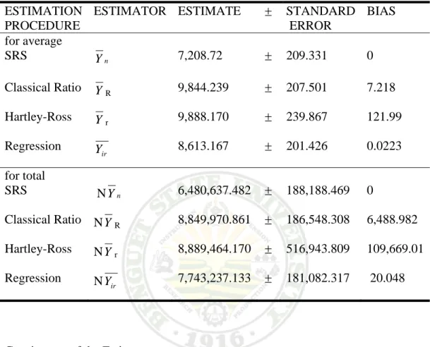
The estimates of the mean and total production of strawberry using the four estimators are presented in Table 1. It showed that simple random sampling had the least estimated mean that is about 7,208.718 grams and a total of 6,480,637.482 grams in estimating strawberry production. Hartley-Ross estimation had the largest mean and total estimation that is about 9,888.170 grams and 8,889,464.170 grams. Classical estimation had 9,844.239 grams estimated mean and 8,849,970.861 grams estimated total production while regression estimation had the largest mean and total estimation that is about 9,888.170 grams and 8,889,464.170 grams. Classical estimation had 9,844.239 grams estimated mean and 8,849,970.861 grams estimated total production while regression estimation has 8,613.167 grams and 7, 743.133 grams estimated mean and total production of strawberry per plot in Strawberry Farm.

According to Cochran (1977) simple random sampling is a method of selecting n units out of the N such that every one of the _NC_n distinct samples has an equal chance of being drawn. He stated also that Ratio estimate is consistent. It is biased except for some special types of population, although the bias is negligible for large samples.

Table1. Estimates of mean and total of Strawberry Production using four methods of estimation.

ESTIMATION PROCEDURE

ESTIMATOR ESTIMATE ± STANDARD ERROR

BIAS for average

SRS _Yn 7,208.72 ± 209.331 0

Classical Ratio YR 9,844.239 ± 207.501 7.218

Hartley-Ross Y_r 9,888.170 ± 239.867 121.99

Regression

Yir 8,613.167 ± 201.426 0.0223

for total

SRS NYn 6,480,637.482 ± 188,188.469 0

Classical Ratio NYR 8,849,970.861 ± 186,548.308 6,488.982 Hartley-Ross NY_r 8,889,464.170 ± 516,943.809 109,669.01 Regression NY_ir 7,743,237.133 ± 181,082.317 20.048

Consistency of the Estimates

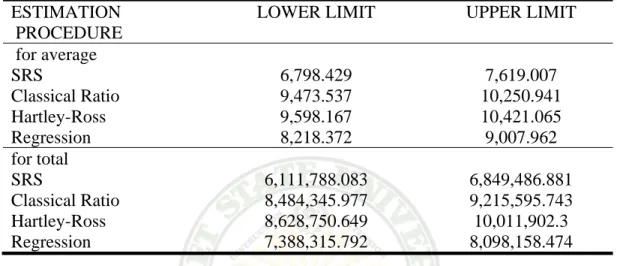
Table 2 shows the Confidence Interval of the true mean and total of the strawberry production using the different estimation procedures. Result shows that Hartley-Ross ratio-type has the largest 95% Confidence Interval for the true mean with a value of 9,598.167 grams to 10,357.957 grams and true total with a value indicated to be 8,467,126.872 grams to 9,311,802.788. Simple random sampling, a biased estimator has the least confidence interval for true mean with a

values of 6,798.429 to 7,619.007 grams and total production of 6,111,788.083 grams to 6,849,486.881 grams. Moreover, for the bias estimators, regression

Table 2. Confidence Interval of the true mean and total strawberry production using three methods of estimation

ESTIMATION PROCEDURE

LOWER LIMIT UPPER LIMIT

for average

SRS 6,798.429 7,619.007

Classical Ratio 9,473.537 10,250.941

Hartley-Ross 9,598.167 10,421.065

Regression 8,218.372 9,007.962

for total

SRS 6,111,788.083 6,849,486.881

Classical Ratio 8,484,345.977 9,215,595.743

Hartley-Ross 8,628,750.649 10,011,902.3

Regression 7,388,315.792 8,098,158.474

estimator has the least confidence interval with 8,218.372 to 9,007.962 for the true mean and 7,388,315.880 to 8,098,158.386 for the true total production.

Precision of the Estimates

The study of Damoslog and Tomin (2007) showed that classical ratio estimator with the least variability is the more precise estimator. Table 3 showed that classical ratio estimation had the least variability with 2.108 is the more precise estimation but regression estimator also had a close value of coefficient of variation which is 2.339. Specifically, simple random sampling has the highest coefficient of variation with a value of 2.904 compared to the other estimators. It was also found that the different estimators have small variability with Hartley

Ross ranked second from the highest variability obtained followed by regression with 2.339 coefficient of variation.

Table3. Coefficient of Variability of the four methods of estimation.

ESTIMATION COEFFICIENT OF

PROCEDURE VARIATION

SRS 2.904

Classical Ratio 2.108

Hartley-Ross 2.720 Regression 2.339

Efficiency of the Estimates

This is supported by Cochran (1977) as cited by Beligan (2004). If oˆ₁and ˆ2

o are unbiased estimators for the parametersθ, that is E(oˆ₁) = E(oˆ₂) = θ, then ˆ1

o is more efficient than oˆ₂ if V(oˆ₁) < V(oˆ₂).

In the study of Damoslog and Tomin (2007), an estimator with higher relative efficiency is considered an efficient Thus, in the said study classical ratio was efficient compared to simple random sampling.

Based from the mentioned criterion for efficient estimators, regression is the most efficient estimators in estimating strawberry production with a variance of 40,572.592 and higher relative efficiency as shown in Table 4. Hartley-Ross ratio-type having a value of 57,449.827 has the largest variance in estimating strawberry production and classical ratio is next to the regression estimation with a variance of 43,189.421.

And this result is the same with the study of Barrios (1995) where regression estimator was considered efficient in estimating socio-economic indicators.

Table 4. Relative Efficiency and Variance of the different estimates compared to simple random sampling.

RELATIVE VARIANCE

PROCEDURE EFFICIENCY

SRS

Classical Ratio 101.77 43,189.421

Hartley-Ross 76.274 57,449.827

Regression 108 40,572.592

SUMMARY, CONCLUSION AND RECOMMENDATION

Summary

The study was conducted to determine the efficiency and consistency of ratio and regression estimation in estimating the strawberry production in Strawberry farm at La Trinidad, Benguet over the simple random sampling method.

The data was gathered from the 29^th day of December 2007 until 3^rd day of February 2008 wherein the researchers ask permission from the owner of the strawberry that was selected as one of the study site. The sample plots were determined using simple random sampling and there were about 195 plots considered. The data gathering ended until the sixth harvesting of strawberries.

The production was estimated using simple random sampling classical ratio estimation, Hartley-Ross ratio-type and regression estimation. It was found that each estimated values obtained due to different estimation schemes utilized.

The classical ratio, Hartley–Ross ratio-type and regression estimators have greater estimated mean and total than the simple random sampling. The regression estimator was said to have the least bias while the classical ratio was considered to have the most bias. Though simple random sampling estimator is not bias, it is considered as a consistent estimator since its 95 % confidence interval for the true mean and true total of the strawberry production is narrow. Among the considered bias estimator, regression was more consistent with its 95 % confidence interval

which is limited or having the least confidence interval. Classical ratio estimate is also considered as the most precise among the estimates since it has the lowest coefficient of variation. Result of the relative efficiency shows that regression estimator is the more efficient compared to simple random sampling.

Conclusion

It is therefore concluded that classical ratio estimator is the most precise among the four different estimators used in estimating strawberry production with its least coefficient of variability. Moreover, simple random sampling was a consistent and unbiased estimator.

However, regression estimator is the most efficient and most consistent among the bias estimators as applied to strawberry production.

Recommendation

It is recommended that some study has to be conducted using the independent variable that is the number of plants per plots to determine the efficiency of estimator for more meaningful estimate .To maintain a high degree of precision, the variability among sampling units within a plot should be kept small. It is also recommended that in estimating strawberry production it is efficient to use the regression estimator over simple random sampling.

LITERATURE CITED

BARRIOS, E. B. 1998. Small area Estimator of Employment Rate.7^th National Convention on Statistics. Manila, Philippines.

BELIGAN, S.Z. 2004. Survey and Sampling Techniques Syllabus COCHRAN, G. W. 1997.Sampling Techniques.3^rd Edition. John Wiley and Sons,

United States of America.

DAMOSLOG, F.T. AND TOMIN, J.T. 2007. Efficiency of Ratio and Regression Estimator s in Estimating Farmers’ Income in La Trinidad Benguet.

DENG, LI-YUAN AND CHHIKARA.R.S (1990). On the Ratio and Regression Estimation in Finite Population Sampling

DORFMAN, J.H. AND SANDERS, D.R. 2004. Generalized Hedge Ratio Estimation with an unknown model

EVERITT, B.S. 1998. Dictionary of Statistics.

FAEDI W., MOURGUES F AND ROSATI. Strawberry Breeding and Varieties:

Situation and Perspective

HSU AND KUO. 2000. Household Solid Waste Recycling Included Production.

LOHR,S.L.1999. Sampling:Design and Analysis.Brooks/Cole PublishingCompany

M.GOSSOP, J.STRANG, P.GRIFFITHS, B.POWIS AND C.TAYLOR. Drug Transitions Study, National Addiction Centre, Maudsley Hospital, London

ONATE, B.T.1967. Ratio Estimators in Field Research. The Philippine Statistician

Vol.VXI, No.3-4:62-74

(Oxford Quick Reference)Dictionary

PALANISWAMY, U.R AND PALANISWAMY, K.M.(2006). Handbook of Statistics for teaching and research in plant and crop sciences.

RAND CORP SANTA MONICA CALIF. Some Finite Population Unbiased Ratio and Regression Estimators.

SUKHATME, B.V. Hartley-Ross Unbiased Ratio-Type Estimator

TOTEMIC N. All season Strawberry Growing with day-neutral Cultivars.

WALPOLE, R.E.ET.AL.1998. Probability and Statistics for Engineers and Scientists.Prentice-Hall, Inc.6th edition.

WEI CHEN, YOSHINAO OOEDA AND TOMONORI SUMI. 2005. A study on a shopping Frequency Model with the Consideration of Individual Difference. Kyushu University, Japan.

Appendix A. Application for Oral Defense

Benguet State University College of Arts and Sciences

DEPARTMENT OF MATHEMATICS-PHYSICS-STATISTICS APPLICATION FOR ORAL DEFENSE

Date: March 17, 2008 Group Members:

Emily June C. Alos Major: Statistics

Eleonor B. Bat-oy Minor: Information Technology Degree: BACHELOR OF SCIENCE AND APPLIED STATISTICS

Title of Thesis: “Efficiency of Ratio and Regression Estimation in Estimating the Strawberry Production.”

ENDORSED BY : MARYCEL H. TOYHACAO Adviser

Date and time of Defense: March 18, 2008 @ 5 PM Place of Defense: CAS Annex 210

NOTED BY : MARIA AZUCENA B.LUBRICA Department Chairman REPORT OF RESULT ON ORAL DEFENSE

Name and signature *Remarks

Marycel H. Toyhacao _______________________

Adviser

Salvacion Z. Beligan _______________________

Member

Maria Azucena B.Lubrica _______________________

Member

Cristina B.Ocden _______________________

Member

*passed or failed

Appendix B. The raw data of strawberry production

Harvesting

plots 1st 2nd 3rd 4th 5th 6th Production(g) # of plants 1 1000 700 700 1000 1700 1100 6200 120 2 1000 600 800 500 1700 1100 5700 116 3 1000 900 500 600 1100 1200 5300 114 4 1000 500 1300 900 1900 1800 7400 122 5 700 700 800 500 900 1000 4600 110 6 800 700 900 600 1600 1250 5850 110 7 1000 500 1100 900 1700 1600 6800 122 8 1000 300 1000 1000 1300 1400 6000 118 9 1000 600 1100 1500 1200 1100 6500 116 10 700 500 600 1500 1200 1500 6000 116 11 700 400 700 1000 1100 1600 5500 118 12 700 600 800 1200 1300 1300 5900 120 13 600 400 1000 1000 1300 1250 5550 136 14 600 600 600 500 1400 1100 4800 110 15 1200 600 600 900 1200 1600 6100 112 16 600 600 700 500 1400 1750 5550 112 17 600 600 600 1100 1250 1900 6050 101 18 500 500 900 1200 1700 1100 5900 112 19 700 200 900 1500 2300 1150 6750 118 20 500 600 800 800 1700 1900 6300 120 21 600 400 800 700 1300 1800 5600 118 22 700 400 900 900 1400 1400 5700 112 23 600 400 900 1700 1450 1450 6500 110 24 700 400 900 1700 1950 1000 6650 108 25 600 300 800 1400 1850 1100 6050 110 26 600 500 900 1800 1500 1150 6450 112 27 500 300 900 1400 1900 1250 6250 106 28 600 500 600 1700 1500 1000 5900 130 29 700 500 900 1700 1850 900 6550 114 30 600 600 600 1600 1700 1800 6900 112 31 500 500 800 1600 1700 1800 6900 114 32 500 500 500 1600 1450 1900 6450 110 33 700 300 1200 1300 1700 1100 6300 114 34 500 300 700 1350 1450 1200 5500 106 35 600 300 800 1250 1500 1000 5450 110 36 400 300 700 1000 1700 1700 5800 130 37 400 500 800 1600 1200 1600 6100 108 38 900 500 1100 600 2250 1850 7200 110 39 600 400 1000 1400 1900 1550 6850 104 40 300 800 900 600 1300 1250 5150 106 41 500 200 700 600 900 1900 4800 124 42 300 100 400 800 1100 1800 4500 106

43 600 400 800 400 300 1000 3500 118 44 400 600 600 400 500 1150 3650 120 45 400 500 900 500 500 1100 3900 106 46 500 400 400 300 500 1000 3100 108 47 600 300 700 300 400 1500 3800 106 48 700 800 100 400 400 1000 3400 108 49 300 600 1000 400 500 800 3600 106 50 500 300 1200 500 500 1100 4100 94 51 400 400 700 400 300 1250 3450 108 52 300 500 900 300 300 1200 3500 104 53 400 700 900 500 500 800 3800 108 54 700 200 600 200 300 900 2900 110 55 500 600 500 200 300 1150 3250 106 56 400 400 700 300 400 800 3000 108 57 400 400 600 400 400 850 3050 118 58 400 600 700 200 400 1050 3350 116 59 600 700 600 300 300 850 3350 110 60 500 300 700 400 500 700 3100 108 61 800 900 800 500 500 1350 4850 108 62 400 400 600 400 400 800 3000 106 63 400 200 400 400 500 1250 3150 110 64 400 300 400 200 300 1000 2600 112 65 200 200 300 200 200 1000 2100 120 66 400 500 300 300 300 1100 2900 130 67 150 200 200 300 400 1150 2400 118 68 250 250 300 100 200 800 1900 114 69 200 300 400 200 200 1150 2450 116 70 400 300 200 100 300 1000 2300 122 71 200 300 400 300 400 1250 2850 120 72 500 300 300 300 500 800 2700 120 73 400 300 300 300 400 800 2500 124 74 300 400 500 200 100 900 2400 126 75 200 500 200 400 300 950 2550 130 76 300 500 200 100 100 850 2050 126 77 300 300 200 300 400 800 2300 128 78 200 400 500 400 300 1000 2800 129 79 300 300 200 200 400 1100 2500 132

80 600 500 700 700 500 1150 4150 130 81 500 900 900 900 900 800 4900 128 82 300 900 900 900 800 700 4500 122 83 1300 17000 900 1100 1200 2000 23500 115 84 1100 8000 900 1400 1400 2100 14900 96 85 1600 1000 500 1000 1600 2000 7700 116 86 1200 900 300 1000 1000 1500 5900 114 87 11100 1000 1200 1500 1900 2200 18900 123 88 1200 1000 600 1400 1600 2000 7800 120