These are part of the unedited lecture notes for a complexity course taught between 2001 and 2010 at NUS, Singapore. These notes, which are copyrighted by the author, may be used by individuals for non-commercial, educational purposes.
Overview
An often-cited concept is that of emergence, which refers to the emergence of laws, patterns, or order through the cooperative effects of the subunits of a complex system. It is the apparent universality of the laws of physics, for example, that makes the world intelligible and gives us confidence in its ultimate simplicity.
Examples
- Schooling of Fish
- Bacterial Colonies
- Forest Fires
- The Double Pendulum
- The Leopard Spots
See the figures showing the number of fires in function of the area burned, in different regions of the United States of America and Australia. For larger oscillations, the motion of the simple pendulum is still periodic, but is no longer given by a simple formula.
Summary
Later in this course we will look at many other interesting systems that are far from equilibrium, some of which exhibit cyclic behavior.
Exercises
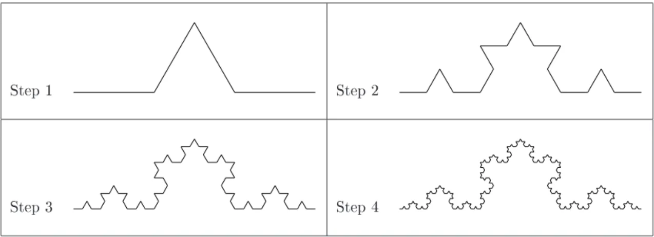
The Koch Curve and Snowflake
Therefore, the length of the prefractals diverges as the number of steps increases, leading to an infinite length for the Koch curve. Alternatively, one can start with an equilateral triangle and apply the Koch curve generator repeatedly to each line segment.
Dimensions
So if a smooth curve can be covered using N units of that measure, the length of the curve can be estimated as N s. As the size of the measuring stick is changed, the total length of the curve changes, as we saw for the Koch curve.
Random Fractals
Random fractals can be generated by modifying the iteration process in the last section to include a probability element. The initiator and generator are as before, but in the following steps (k= 2 onwards) the prefractals are obtained by replacing each line segment with the generator in such a way that the triangle of the generator points randomly (e.g. determined by a coin toss) to each side of the original line.
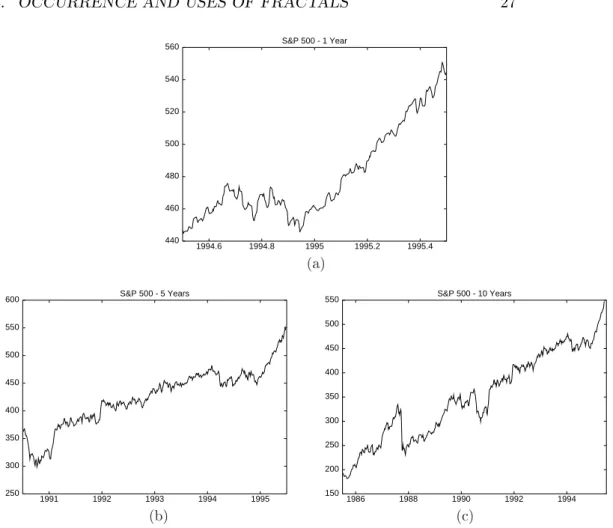
Occurrence and uses of Fractals
Note that the equation above is of the same form as that given from the definition of the self-similarity dimension above. Remember from the example of the Koch curve that one can accommodate long lengths in small.

Dynamical generation of some random fractals: Diffusion Lim-
The location of the next step is generated e.g. of two random numbers which respectively give the direction (angle) and length of the walk. Another dynamic 'explanation' for the ubiquitous occurrence of fractals and power laws in nature is the idea of 'self-organized criticality', which we will discuss later in the course.

Scaling Laws in Biology
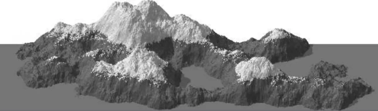
Fractals and Art
Summary
Exercises
What is the area of the Koch snowflake if the initiator was an equilateral triangle of unit length on each side. Calculate the self-similarity dimensions of the Koch curve using the scales s= 1/9 and s= 1/27. a) Give examples of objects that are the same over a wide range of scales, but which are not fractals.
Some of the figures (those with a copyright notice in small print in the figure caption) used in this chapter are from the website of Ref.[1] taken. while some other figures used in the lectures are taken from Refs[3,4]. When meteorologist Edward Lorenz studied a simplified model of the weather, he discovered that small differences in the initial conditions quickly led to very different final results.
Dynamical Systems and Iterative Maps
A Simple Example of an Iterative Map
An Intuitive Analysis
A SIMPLE EXAMPLE OF AN ITERATIVE MAP 37 A mechanical analogy of the two fixed points, stable and unstable, is a ball lying at the bottom of a valley and one lying on a hilltop. Both positions of the ball are points of static equilibrium, but one position is clearly stable while the other is not.
A Graphical Analysis
Moreover, the stability of the ball at the bottom of the valley is limited to perturbations that do not cause the ball to pass over a nearby peak, and therefore in general the basin of attraction of a stable equilibrium point is of limited extent . Since the period-one fixed points correspond to the solutions of xn+1 = xn, graphically these can be found by intersecting the map function y = f(x) with the straight line y = x.
The Analytical Approach
A SIMPLE EXAMPLE OF AN ITERATIVE MAP 39 Since the above fixed points correspond to a situation where the future values of x remain the same at each time step, they are called period one fixed points. For the case f(x) =x2, the intersections are at the origin and prix= 1, as we already know.
A Discrete Model of Population Growth
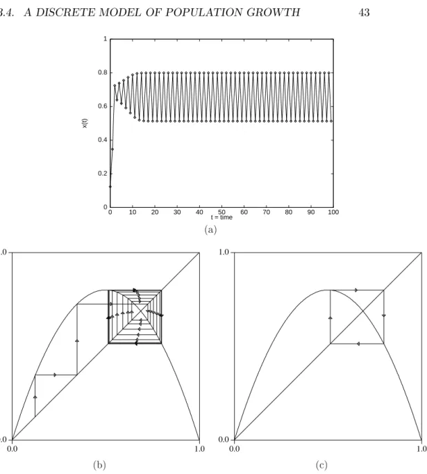
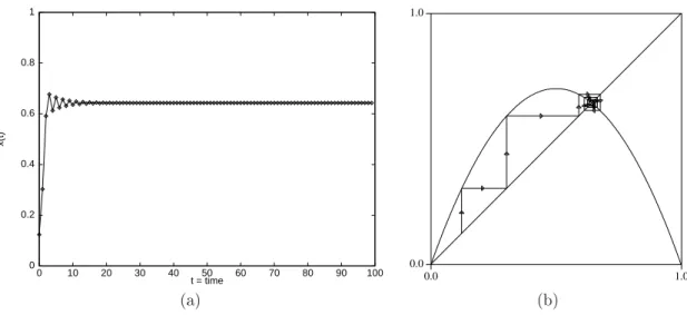
Varying the control parameter in the logistic map
That is, the origin is the only fixed point for 0≤r≤1/4 and is attractive (stable) for all x0. As the state space plot in Figure (3.3b) confirms, the fixed point at the origin is now unstable and the system is attracted to a new stable fixed point from period one.
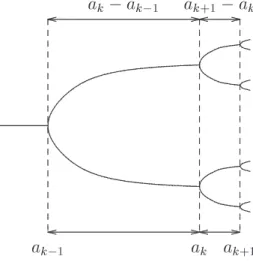
Bifurcation Diagrams
As r increases further, these odd periodic attractors themselves undergo period-doubling bifurcations into chaos. The self-similarity is also important in establishing some universality properties of the bifurcation process, as discussed below.
The Feigenbaum Constant and Universality
The actual proof of this statement is quite involved, but in short it uses the concept of the renormalization group that was developed to deal with critical phenomena in statistical mechanics. Although Eq.(3.18) is defined in the limit k → ∞, it can be used to estimate the point at which a system becomes chaotic, a∞, if the first few bifurcations of the system are known.
Experimental Tests
Although the discussion so far has been strictly limited to the logistic map, the constant δ is the same for other smooth one-dimensional maps with a single hump. THE ROSSLER SYSTEM 51 details of the actual experiments which are dynamical systems with many de-.
The Rossler System
The behavior of the z variable in the chaotic state (c= 5) is illustrated by looking at the time series shown in figure (3.12a). From that, you see that the z-coordinate is small most of the time, which means that the trajectories are mostly close to the x−y plane.
The Lorenz map
For the Rossler system in the chaotic state, e.g. c = 5, the time series for the x-variable is shown in Fig. (3.12b). However, not all systems have a one-dimensional Lorenz map, as this requires the system's strange attractor to be nearly flat.
Noise versus Chaos
For attractor reconstruction to be successful, there are two issues that must be addressed.
Summary
In the previous chapter we saw how the geometric complexity of nature can be described by simple algorithms and models that generate fractal structures. However, the apparent disorder is chaotic rather than random, as the order is now hidden in the phase space of the system.
Exercises
Use the critical values of the control parameter for the logistic map, ak, given in the text to estimate. Use your favorite software (eg maple file ross.mws) to explore the Rossler system (time series and phase plots) for different values of the control parameter c.
State Variables
In addition to the temperature, one may need more thermodynamic parameters, called state variables, to fully characterize the state of the system. Variables such as temperature and pressure that are independent of the size of the system are called intensive, while those such as volume are called extensive.
The Ideal Gas
Hence the net change in momentum is -2nmAvx2 dt and hence the pressure F/applied by the piston on the gas is -2nmv2x and so the pressure of the gas is by Newton's third law. For a monatomic gas, < mv2/2 > is the average kinetic energy of an atom, and the quantity N < mv2/2> thus represents the total internal energy U of the gas.
Statistical Mechanics
Ergodic theorem: After a sufficiently long time, each representative point of the system will cover the entire accessible phase space. That is, entropy is a measure of the total number of different microscopic states in which the macroscopic system can exist.
The Second Law
In the example above, the probability that a molecule is in the left half of the box is 1/2. Thermodynamically, one says that time flows in the direction of increasing entropy, or the arrow of time is in the direction of increasing entropy of the universe.
The First Law
Looking around, we see that most of the changes in the universe lead to an increase in randomness and are irreversible.
Entropy for Open Systems
On the other hand, the entropy S can be treated as a function of U and V (see the statistical definition given earlier), which changes under an infinitesimal reversible transformation with . If you look at the change in entropy of the combined larger system of gas plus reservoir, it is zero, in accordance with the second law (for isolated systems).
Phase Transitions
Second Order Transitions
In the high temperature phase the system is disordered, with no net magnetization, but with complete rotational symmetry (isotropy). When M = 0 one is in the high-temperature disordered phase, while for M 6= 0, one is in the low-temperature ordered phase with net magnetization.
Correlation Function and Critical Exponents
Critical Opalescence
As the temperature is increased, more of the liquid will evaporate, rapidly increasing the density of the gas phase. In the table, the experimental values of the scaling relations are compared with the theoretical predictions.
Scaling Laws
The Ising Model
Although the Ising model is simple to state, the calculation of its thermodynamic properties is extremely complex and ford= 3 requires numerical effort using a computer. Nevertheless, many other models, as simple as the Ising model but different from it, have been used to model real systems and to calculate and compare their critical properties.
Percolation
That is, although the spins only interact with their neighbors, the net result can be a cooperative state, in which far-distant spins are correlated. Quantitatively, it is remarkable that such a crude model gives theoretical predictions for the critical exponents and scaling relations that are consistent with experiments on real systems.
Summary
More commonly cited examples of universal emergent laws are those that arise near the critical point of a second-order phase transition. Percolation is a geometric analogue of thermal systems that exhibits behavior similar to that of second-order phase transitions.
Appendix
The Scaling Hypothesis
If a quantity is dimensionless (for example, fractional volume), it remains unchanged when the length scale is changed. The scaling hypothesis suggests that near the critical point the correlation length, ξ, is the only characteristic length scale in terms of which all other quantities must be measured with length dimensions.
Exercises
The entropy of a thermally isolated system never decreases (ie restore the original statement of the second law in the text). Make sure that the above extreme principles are equivalent in limited cases to the first version of the second law given in the text. a) Show that both sides of equation (4.27) have units of thermal energy.
Power Laws in Nature
On the other hand, the aforementioned systems exhibit a scale-free behavior similar to that exhibited by equilibrium systems near the critical point of the second-order phase transition. It is important to note that while the critical state in a second-order equilibrium phase transition is unstable (slight perturbations move the system away from it), the critical state of self-organized systems is stable: it constantly attracts the systems.
Models
Although the effect of adding any particular grain is almost impossible to predict, the statistical distribution of avalanches according to an approximate inverse power law implies that small avalanches are more frequent than larger ones. Thus it has been suggested that self-organized criticality may be not only the reason for the various power laws in nature, but also the dynamical mechanism behind fractal geometry and one-over-f time phenomena (see Chapter 2).
Experiments
Note that a key feature of the models, which is a reflection of real systems, is that the external process that drives the system (inflow) occurs much more slowly than the faster internal reorganization processes that cause dissipation.
Life
War and Peace
Zipf’s Law
Summary
Exercises
What evidence is there that wildfires are an example of a self-organized critical system. Can you justify your answer in (c) in the light of claims of self-organized criticism of the system. e) Check Ref.[9] and others similar in spirit.
Check out the websites below of Zipf's Law. a) Find other situations where Zipf's law applies.