I understand that a copy of my research will be deposited in the University Library for permanent storage. I understand that the British University in Dubai may make a digital copy available in the institutional repository.
Introduction
- Background
- Significance of the Study
- Aims and Objectives
- Research Questions
- Thesis structure
Is there a difference between the volatility of green and mainstream bond markets? The purpose of this paper is to understand the conditional volatility of the green and conventional bond market.
Green Bonds Market Overview
- Introduction
- The Beginning of the Green Bonds Era
- The Green Bonds Principles
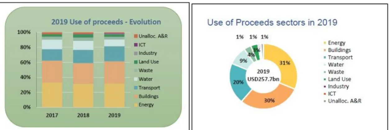
- Use of Proceeds
- Process for Project Evaluation and Selections…
- Management of Proceeds
- Reporting
- SWOT Analysis
- Strengths
- Weaknesses
- Opportunities
- Threats
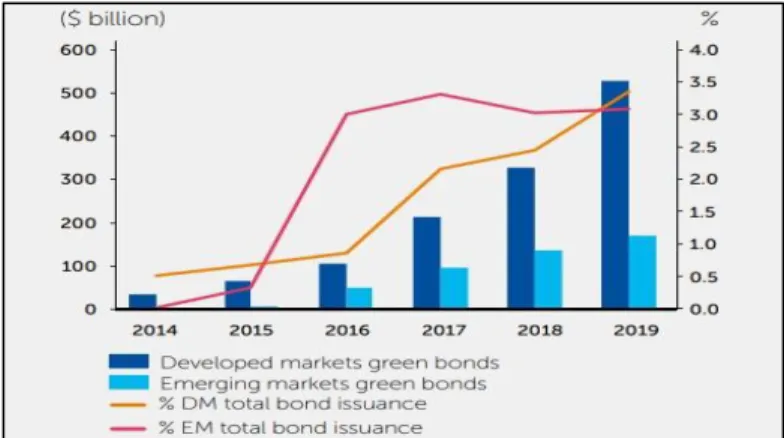
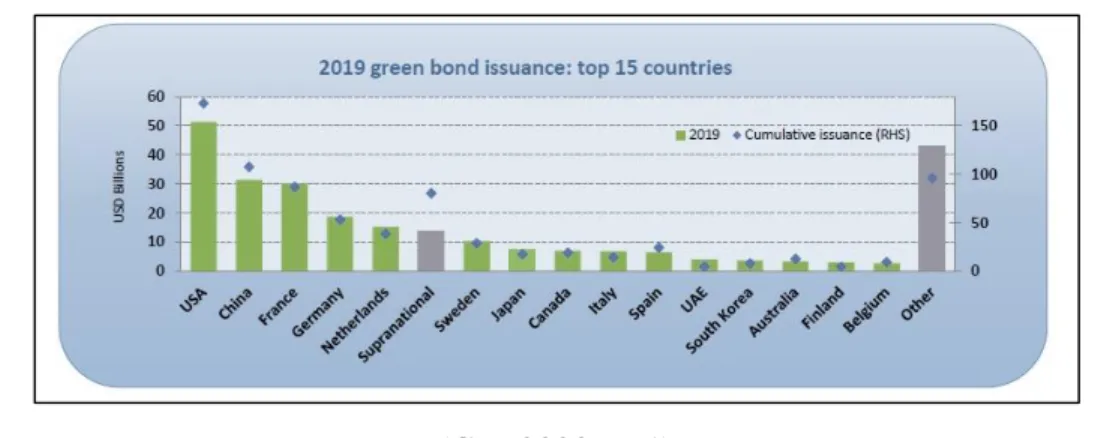
- Green Bonds Market in 2020
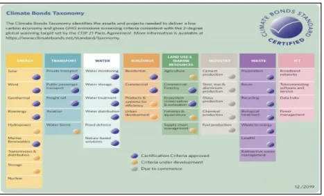
This principle requires green bond issuers to appropriately track the proceeds of green bonds. As a result, if not properly monitored, the credibility of the green bond market could be seriously adversely affected.
Literature Review
- Introduction
- Green versus Conventional Bonds Literature
- Multivariate GARCH Model Development
- What is GARCH?
- What is MGARCH?
- DCC Multivariate GARCH Applications Across Markets
- Research Hypothesis
- Research Gap
The researchers found that there is evidence that both green and non-green bond markets experience sensitivity to certain macroeconomic variables. Moreover, they found that across the entire selected sample, the yield premium is on average -2 basis points for the green bonds compared to the non-green. The research found that this lower return in the green bonds is seen more in the financial bonds and those with a low rating.
However, they wanted to test whether green and non-green bonds are priced differently. Hachenberg and Schiereck (2018) concluded that, on average, green bond trading is not very different from conventional bond trading. In addition, the researchers conclude that green bonds issued by governments are traded more than comparable conventional bonds.
2018) conducted a study analyzing the impact of liquidity risk on yield spreads for green and non-green bonds. The researcher concluded that the green bond market has a significant movement with the fixed income market, i.e. applying the Value-at-Risk (VAR) and Conditional Valua-at-Risk (CoVaR) approach, the study concluded that the market for green bonds is experiencing significant price spillovers from the fixed income market.
Econometric Methodology
- Introduction
- DCC Multivariate GARCH
- Data
- Bloomberg Barclays MSCI Global Green Bond Index (GB)
- Bloomberg Barclays Global Aggregate Total Return Index (CB)…
- Weekly returns
- Descriptive statistics
- Normality Test
- Preliminary Tests
- Stationarity Test
- Volatility Clustering Test
- Autocorrelation Test
- First Step: Selecting the Best Univariate GARCH Model
- Selecting ARMA (p,q) Orders
- Choosing the best ARMA Model
- White Noise Testing
- Testing Symmetric and Asymmetric GARCH Models
- Selecting the best GARCH Model
- Second Step: Estimating the DCC GARCH Model Parameters
- Dynamic Conditional Correlations
- Volatility linkages
- Structural Break
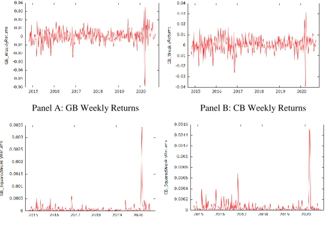
The first stage is to estimate the volatility of the green bond market index and the conventional bond market index using different types of univariate GARCH models. Moreover, as stated in "Environmental-Finance" (2020), the GB index has been selected as the best index for the last four years and for the year 2020. Moreover, the standard deviation of the GB and CB indices says that the experience of GB 0.9% deviation from the mean and CB experience 0.7% deviation from the mean.
This section presents the steps that lead us to determine the best type of univariate GARCH model for modeling the volatility of each of the time series. The selection of the best model depends on having the lowest Akaike Information Criterion (AIC). Once we have the results, we check for normality of the standardized residuals by assessing skewness, kurtosis and the Jarque-Bera test.
Based on the normality results of the standardized residuals, we run the DCC-GARCH model using STATA statistical software using either Maximum Likelihood or Quasi Maximum Likelihood. Understanding when a structural break occurred provides insight into the behavior of the data in question. First, we will need to determine the date of the sudden change in the pattern.
Results and Discussion
Introduction
Normality Test for the Data Set
This paper will later perform a normality test on the standardized residuals to determine whether to use the Maximum Likelihood (ML) or Quasi-Maximum Likelihood (QML) estimator.
Preliminary Tests
- Stationarity Test
- Volatility Clustering Test
- Autocorrelation Test
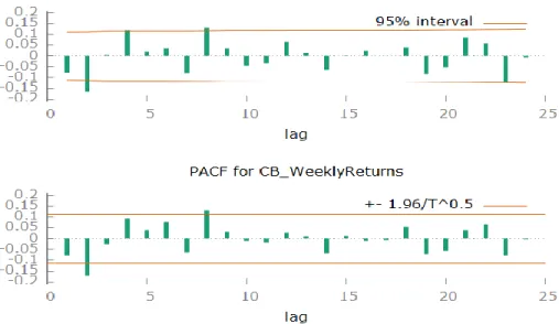
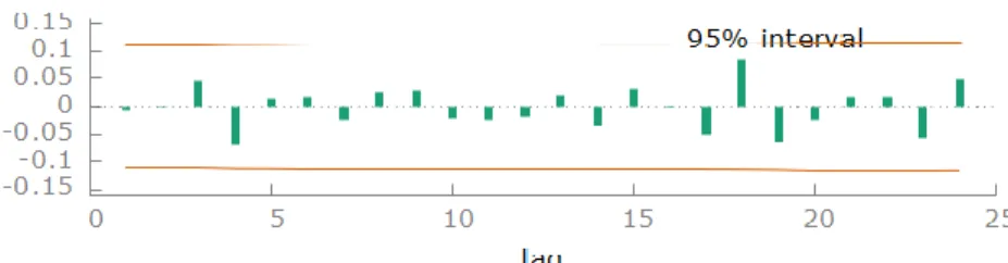
On the other hand, using equation (8), the returns of GB and CB are stationary as the p-value is less than 1% level of significance. In Figure 7, we can also see that the returns of GB (Panel A) and CB (Panel B) have an average that returns. Figure 7 shows the time series plot for the GB and CB returns and quadratic returns.
Indeed, Cont (2007) stated that the returns of financial time series data often show volatility clustering. Panels A and B present the weekly returns of GB and CB, while panels C and D present the weekly squared returns. The Ljung-Box test for autocorrelation results of returns and squared returns are presented in Table 5.
While the p-values for returns and squared returns are statistically significant for both bonds, the squared returns were more significant. The high level of significance of returns and squared returns also numerically support the fact that both indices experience volatility clustering, as discussed in the previous section. In conclusion, since the weekly returns of the Bloomberg Barclays MSCI Global Green Bond Index (GB) and Bloomberg Barclays Global Aggregate Total Return Index (CB) are first-order stationary, clustering volatility, ARCH effect and autocorrelation, we can conclude that a The GARCH model can be applied to model the data for both variables (Park, Park and Ryu 2020).
First Step: Selecting the Best Univariate GARCH Model
- Selecting ARMA (p,q) Orders
- Choosing the Best ARMA Model
- White Noise Test
- Testing Symmetric and Asymmetric GARCH Models
- Selecting the best GARCH Model
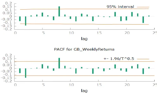
From the table, we find that the ARMA (8,8) model has the lowest AIC value for both indices, GB and CB. Therefore, in our case, to ensure that ARMA (8,8) accurately captured all available information in GB and CB, Figure 9 presents their correlogram to show the results of the white noise test on the model residuals. Therefore, this paper will accept the null hypothesis that GB and CB exhibit white noise in the residuals of their ARMA (8,8) model.
This means that the residuals of the ARMA (8,8) model for the mean equation in the GARCH are random and independent. Based on the lowest AIC value from Table 7, the best GARCH model to examine the volatility of GB and CB is the standard symmetric GARCH model. It is worth noting that since we chose the GARCH model, then we assume that negative and positive shocks have the same impact on GB and BQ (Lahrech 2019).
For CB, it is evident that all coefficients in the conditional mean equation are statistically significant at 1% and 5%. Looking at the coefficients of GB and CB for 𝛼1 side by side, we can see that GB has a higher value than CB. On the other hand, the coefficients of 𝛽1 for GB and CB show that GB has a lower value than CB.
Second Step: Estimating the DCC GARCH Model Parameters
- Normality Test for Standardized Residuals
- DCC-GARCH Model Results
- Dynamic Conditional Correlations
Note: 𝜔 is for constant, 𝜑𝑖 is for AR, 𝜃𝑖 is for MA, 𝛼𝑖 is for ARCH terms, 𝛽1 is for GARCH terms. In this case, this paper will continue to estimate the DCC-GARCH model using the maximum likelihood estimator. Looking at the results, we find that the ARCH and GARCH terms for GB and CB are all statistically significant at 1%.
In other words, we can say that there is a short-term volatility spillover between GB and CB. Note: 𝜔 is for constant, 𝑎1 and 𝑎2 are for ARCH terms, 𝑏1 is for GARCH terms. In addition, this paper performs a Wald test to check whether the DCC model should be reduced to CCC for better analysis.
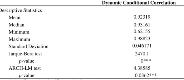
Based on the estimated DCC model, this paper proceeds to estimate the conditional correlation values between GB and CB. This paper finds that the conditional correlations between GB and CB vary over time, are positive, and are on the high side. In addition, we find that the conditional correlations between GB and CB are not normally distributed (Jarque-Bera test) and show heteroskedasticity (ARCH-LM test).
Volatility Linkages
Moreover, using a different methodology, Reboredo (2018) found that the green bond market experiences co-movements with the conventional market. This joint movement is in fact explained by Broadstock and Cheng (2019) who found that both markets are sensitive to the same macroeconomic factors. Hassan et al. 2018) found that when a stressful event occurs, security prices become drastically more volatile, as many investors tend to sell what they consider less liquid and buy safer and more liquid securities.
In addition to the graphical analysis, we investigate the volatility links between GB and CB in a numerical way using the pairwise correlation tool on the univariate GARCH conditional variances. This paper concludes that at a global level, the conditional variance of GB and CB experiences high and strong positive correlation at a value equal to 0.922. This can be attributed to the fact that the green bond is a sub-market of the wider one.
Structural Break
Summary of the findings
Conclusion
- Introduction
- Summary of the Study
- Summary of the Findings
- Implications and Recommendations
- Limitations of the Study
- Future Research Suggestions
Finally, it provided the current state of the green bond market by presenting the top 15 leading countries and its current statistics compared to the previous years. This study looks at understanding whether a dynamic conditional correlation exists between the green bond and the conventional bond markets at a global level. Third, with the exponential growth that the green bond market is witnessing, this article provides market participants with information related to the characteristics of the newly formed market.
This paper will in turn serve as a foundation when it comes to deciding whether or not to allocate funds in the green bond market. Finally, this article recommends policy makers to establish policies, regulations and practices aimed at increasing the differentiating strategies of the green bond market and the conventional bond market in order to attract a wider variety of investors to the green bond market. This paper faced few limitations due to the fact that the green bond market is still in its nascent phase.
First, there was a very limited number of studies examining the characteristics of green bond market volatility. Second, the studies comparing the green bond market with the conventional bond market were conducted on their comfort of issuance, price spread, premiums and interest rate spreads. Third, this paper recommends comparing the volatility of the green bond market and the conventional bond market in the UAE, as it is the only country in the MENA region that has been recognized as one of the top 15 green bond issuing countries.