Click on the ad to read more Click on the ad to read more Click on the ad to read more. Next, susceptibility and permeability are defined, and the boundary conditions on the magnetic and auxiliary fields are derived. To understand the concepts of electric field lines and electric flux as the surface integral of the electric field.
Click on the ad to read more Click on the ad to read more Click on the ad to read more Click on the ad to read more. Click on the ad to read more Click on the ad to read more Click on the ad to read more Click on the ad to read more Click on the ad to read more.
STUDY AT A TOP RANKED
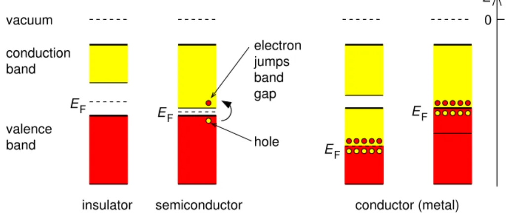
In semiconductors the band gap is small enough that some electrons are able to cross the band gap as a result of thermal excitation and/or in response to an electric field. Semiconductors used to make electronic components are usually "doped" with impurity ions which bring energy levels within the band gap. In a conductor, electrons move in response to an electric field, which in electrostatics is due to other charges, and will continue to move until they reach the surface where they will redistribute until the electric field inside the conductor disappears.
What's going on here is that broken chemical bonds on the surface of a material leave a charge imbalance, and when that material is in contact with another material with a different charge imbalance, electrons will flow from one material to the other. Click on the ad to read more Click on the ad to read more Click on the ad to read more Click on the ad to read more Click on the ad to read more Click on the ad to read more.
INTERNATIONAL BUSINESS SCHOOL
Click on the ad to read more. Click on the ad to read more. Click on the ad to read more. Click on the ad to read more. Click on the ad to read more. Click on the ad to read more. Click on the ad to read more. 1–1 The surface of a non-conducting half-sphere with its center at the origin has a surface charge density σ(a, θ, ϕ) = σ0cosθ and is uniformly charged with a charge of density ρ0. Click on the ad to read more. Click on the ad to read more. Click on the ad to read more. Click on the ad to read more. Click on the ad to read more. Click on the ad to read more. Click on the ad to read more. per ad to read more.
In Appendix E it is shown that the solution of Poisson's equation is unique if V is specified anywhere on the boundaries, or unique up to an additive constant potential if E·n� is specified on the boundaries. Click on the ad to read more Click on the ad to read more Click on the ad to read more Click on the ad to read more Click on the ad to read more Click on the ad to read more Click on the ad to read more on the ad to read more Click on the ad to read more.
CLICK HERE
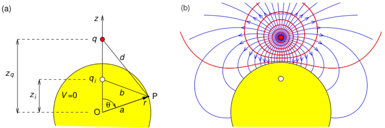
Click on the ad to read more Click on the ad to read more Click on the ad to read more Click on the ad to read more Click on the ad to read more Click on the ad to read more Click on the ad to read more on the ad to read more Click on the ad to read more Click on the ad to read more. Click on the ad to read more Click on the ad to read more Click on the ad to read more Click on the ad to read more Click on the ad to read more Click on the ad to read more Click on the ad to read more on the ad to read more Click on the ad to read more Click on the ad to read more Click on the ad to read more. Then suppose that there is a spherical surface of radius a centered at the origin on which the potential is specified as V(a, θ, ϕ) =V0(θ, ϕ).
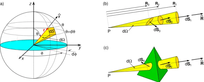
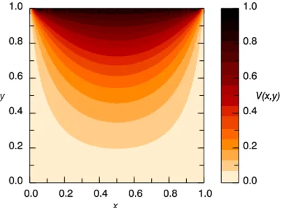
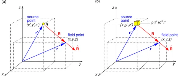
The potential is defined on a rectangular grid with potentials at the boundary points of the grid fixed by the boundary conditions. Consider the potential due to a point charge q on the z axis at a distance r′ from the origin (Fig. 3.1a).
EXPERIENCE THE POWER OF FULL ENGAGEMENT…
Click on the ad to read more Click on the ad to read more Click on the ad to read more Click on the ad to read more Click on the ad to read more Click on the ad to read more Click on ad to read more Click on ad to read more Click on ad to read more Click on ad to read more Click on ad to read more Click on ad to read more Click on ad to read more Click on ad to read more Click on ad to read more Click on ad to read more Click on ad to read more Click on ad to read more Click on ad to read more.
RUN FASTER
Since the monopole and dipole terms are zero, the quadrupole moment tensor is independent of the choice of origin. Click on the ad to read more Click on the ad to read more Click on the ad to read more Click on the ad to read more Click on the ad to read more Click on the ad to read more Click the ad to read more Click on the ad to read more Click on the ad to read more Click on the ad to read more Click on the ad to read more Click on the ad to read more Click on the ad to read more Click on the ad to read more Click on the ad to read more Click on the ad to read more Click on the ad to read more Click on the ad to read more Click on the ad to read more to read Click on the advertisement to read more.
SETASIGNThis e-book
Click on the ad to read more Click on the ad to read more Click on the ad to read more Click on the ad to read more Click on the ad to read more Click on the ad to read more Click on the ad to read more Click on the ad to read more Click on the ad to read more Click on the ad to read more Click on the ad to read more Click on the ad to read more Click on the ad to read more Click on the ad to read more Click on the ad to read more Click on the ad to read more Click on the ad to read more Click on the ad to read more Click on the ad to read more Click on the ad to read more Click on the ad to read more. To know and be able to apply the boundary conditions on the potential, the electric field and the displacement field at an interface between two dielectrics. Click on the ad to read more Click on the ad to read more Click on the ad to read more Click on the ad to read more Click on the ad to read more Click on the ad to read more Click on the ad to read more Click on the ad to read more Click on the ad to read more Click on the ad to read more Click on the ad to read more Click on the ad to read more Click on the ad to read more Click on the ad to read more Click on the ad to read more Click on the ad to read more Click on the ad to read more Click on the ad to read more Click on the ad to read more Click on the ad to read more Click on the ad to read more Click on ad to read more.
There is no surface polarization charge present on the top and bottom surfaces since P·�n= 0 there. There is still negative surface charge on the left side and positive surface charge on the right side, but they have unequal magnitudes: σpol(0, y, z) =−P0 and σpol(L, y, z) = ( P0+aL). Using Gauss' theorem on the 1st integral and E=−∇V on the 2nd integral we find.
In the center of the hole, "O", we must add the field due to the surface polarization charge of the density σpol(θ) on the surface S of the hole,. 4.41). Find: (a) E, D and P everywhere; (b) the polarization surface and volume charge density everywhere, and the net polarization charge; (c) the free charge on the inner and outer conductors and the capacitance. Since the force on section dr of the wire isdFmag=Idr×B, the force on the entire circuit is
Also note that M depends only on the geometry (separation, shapes and sizes) of the two coils. By integrating the torque dN =r′×dF in the line element dr′ of the current circuit atr′, find the torque in the entire current loop. 6.1(c) where on the upper surface Kmag(r) = Mx(y)y which varies according to the position, while on the sides parallel to the x–z plane the current density of the magnetization surface is constant with the values Kmag(x,0 , z).
This scanning electron microscope with polarization analysis (SEMPA) technique can be used to make images of the domain structure on the surface of a ferromagnetic material. SEMPA measurements of the magnetic domains are shown at four points on the hysteresis loop (center), showing the magnetic state corresponding to each image. Another example would be to describe the electric field on the surface of a spherical conductor with beam-carrying chargeq.
After each iteration, the potentials at the outer points of the grid are reset to the potentials at the boundary surfaces.