Particle Physics Reference Library

Others are in the form of the original contribution supplemented by a detailed appendix relating to recent developments in the field. What changed was the nature of the elemental building blocks and new powers were discovered.

Gauge Theories and the Standard Model

Introduction to Chaps. 2, 3 and 4

A good example is that of the measurements of the electroweak mixing angle, discussed in Sect. Updated discussions can be found in the PDG's QCD review, as well as Ref.

Introduction

One topic where things have changed somewhat less is the determination of the strong coupling, discussed in Sect.4.7. In fact, only a subset of the SM symmetry is directly reflected in the spectrum of physical states.

Overview of the Standard Model

Consequently, the measured intensity of the force depends on the transferred (quad)momentum squared, Q2, among the participants. At low energy, the strength of the effective four-fermion interaction of charged currents is determined by the Fermi coupling constant GF.

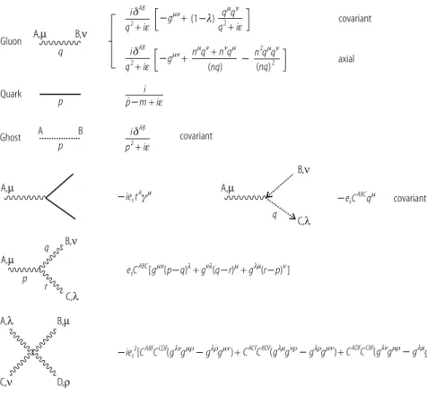
The Formalism of Gauge Theories

and (2.20) it follows that the transformation properties of FμνA are those of a unified representation tensor. In this case, the tensor Fμν is linear in the gauge field Vμ so that in the absence of matter fields the theory is free.

Application to QCD

On the other hand, in the non-Abelian case, the FμνA tensor contains both linear and quadratic terms iVμA, so the theory is non-trivial even in the absence of matter fields. This is reflected in the fact that in QEDFμν is linear in the measurement field, so that the term Fμν2 in the Lagrangian is a purely kinetic expression, while in QCDFμνA is quadratic in the measurement field, so that in FμνA2 we find cubic and quarter peaks beyond the kinetic term.

Quantization of a Gauge Theory

The correct ghost contributions can be obtained from an additional term in the Lagrangian density. The currently accepted method is dimensional regularization [15], which consists of a formulation of the theory of indimensions.

Spontaneous Symmetry Breaking in Gauge Theories

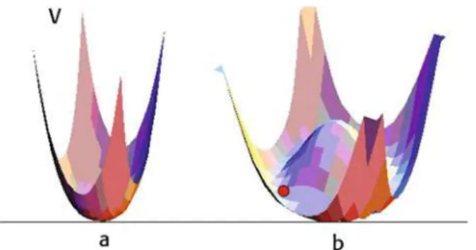
In the quantum case, the classical potential corresponds to tree-level approximation of the quantum potential. So, in the construction of the EW theory we cannot assume massless physical scalar bosons.

Fig. 2.1 The potential V = 1/2 μ 2 M 2 + 1/4 λ(M 2 ) 2 for positive (a) or negative μ 2 (b) (for simplicity, M is a 2-dimensional vector)

Quantization of Spontaneously Broken Gauge Theories

R ξ Gauges

But this mixing term can be eliminated by an appropriate modification of the covariant gauge fixation term given in Eq. 2.65). Also for ξ → ∞ the unitary gauge description returns in that the Goldstone propagator vanishes and the gauge propagator reproduces that of the unitary gauge in Eq.

Images or other third-party material in this chapter are covered under this chapter's Creative Commons license, unless otherwise noted in the credit line for the material. If the material is not covered by a Creative Commons Chapter license and your intended use is not permitted by law or exceeds the permitted use, you will need to obtain permission directly from the copyright holder.

The Standard Model of Electroweak Interactions

Introduction

The Gauge Sector

2YL,RBμ ψL,R, (3.7) where L,RA and 1/2YL,R are the generators of SU (2) and U (1), respectively, in the reducible representations of ψL,R. But in the following we keep tRiψR for generality, in case a non-singlet right fermion is discovered on 1 day.

Couplings of Gauge Bosons to Fermions

In the neutral-current (NC) sector, the photon Aμ and the mediator Zμ of the weak NC are orthogonal and normalized linear combinations of Bμ and Wμ3:. In the same way, we get for neutral currents in Born approximation from Eq. 3.17) the effective four-fermion interaction given by.

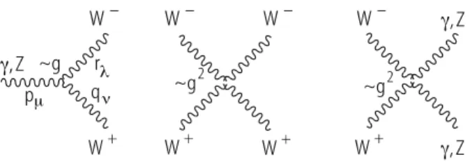
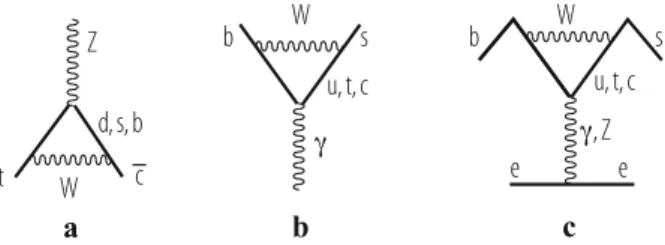
Gauge Boson Self-interactions

In addition to neutrino exchange, which includes only the well-charged current peak, weak gauge triple peaks VW−W+V appear in the γ and Z exchange diagrams. For A = 1 or two we have two charged W and 2W3, each W3 being a combination of γ and Z according to Eq. With a little algebra the quartic vertex can be cast in the form:. where,μdheν refer to W+W+in peak 4W and toV V in case W W V V and:. 3.38).

Fig. 3.3 The three- and four-gauge boson vertices. The cubic coupling is of order g, while the quartic one is of order g 2

The Higgs Sector

In fact, from the Yukawa integrals gφf f¯ (f¯LφfR +h.c.), the mass mf is obtained by substituting φ byv, so that mf = gφf f¯ v. Thus, the trilinear couplings of the Higgs to the gauge bosons are also proportional to the masses.

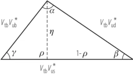
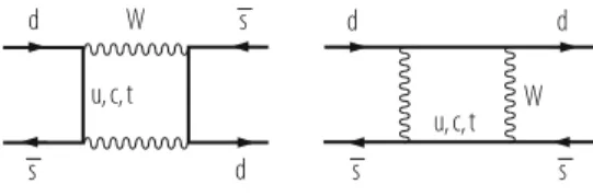
The CKM Matrix

In SM, the non-vanishing of the η parameter (related to the phase ϕ in Eqs. 3.69 and 3.70) is the only source of CP violation. In SM, all CP-violating observables must be proportional to J, therefore to the area of the triangle, or toη.

Fig. 3.6 The unitarity triangle corresponding to Eq. (3.74)

Neutrino Masses

The corresponding mass terms are of the order mν ∼λv2/M, thus of the same generic order of the light neutrino masses from Eq. It is interesting that the observed magnitudes of the mass-squared distributions of neutrinos are well compatible with a scale M remarkably close to the Grand Unification scale, where in fact L non-conservation is naturally expected.

Renormalization of the Electroweak Theory

The pseudo Goldstone bosons w±andza are directly related to the longitudinal helicity states of the corresponding massive vector bosons W± and Z. Thus, the charge of d quarks is −1/3 of the positron charge because there are three colors.

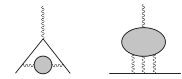
QED Tests: Lepton Anomalous Magnetic Moments

The contribution of the light by light (LbL) scattering diagrams is estimated to be: aLbL.μ. Another puzzle is the fact that using vector current conservation (CVC) and isospin invariance, which are well-established tools at low energy, aμLO can also be evaluated from τ decays.

Fig. 3.10 The hadronic contributions to the

Large Radiative Corrections to Electroweak Processes

Similarly, large logarithms of the form [α/π ln(mZ/μ)]n also appear, for example, in the relationship between sin2θW on the mZ (LEP, SLC) and μ scales (e.g., the scale of low-energy neutral current experiments). This vertex is particularly sensitive to the top quark, which, as a partner of the b quark in a doublet, runs in the loop. Now if they were sufficiently sensitive, we would know exactly the mass of the Higgs.

Electroweak Precision Tests in the SM and Beyond

The Z and W masses must be precisely defined in terms of the pole position in the respective propagators. On the contrary, in the second relation ρm depends on the definition of sin2θW beyond the tree level. As discussed in the next section, these values correspond to the SM with a light Higgs.

Results of the SM Analysis of Precision Tests

The precise determination of the associated final terms would be lost (that is, the value of the mass in the denominator of the argument of the logarithm). In conclusion, the validity of SM has been generally confirmed to a level that we can say was unexpected at the beginning. The impressive success of SM places strong constraints on the possible forms of new physics.

Table 3.1 Summary of electroweak precision measurements at high Q 2 [8]

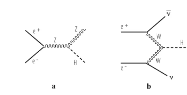
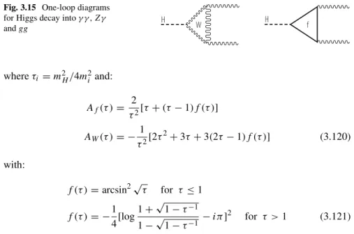
Phenomenology of the SM Higgs

Theoretical Bounds on the SM Higgs Mass
SM Higgs Decays

The big remaining questions concern the nature and properties of the Higgs boson. The exact shape of the experimental upper limit H in SM depends on the value of the upper quark mass. The possible instability of the Higgs potentialV[φ] is generated by quantum loop corrections to the classical expression of V[φ].

Fig. 3.13 The total width of the SM Higgs boson [64]

Limitations of the Standard Model

As discussed in the QCD Chapter (Chap.4), thegg → H vertex provides one of the main production channels for the Higgs at hadron colliders. This so-called hierarchy problem is due to the instability of the SM with respect to quantum corrections. Passarino, The standard model in the making: precision study of the electroweak interactions; Oxford Clarendon Press, (1999).

QCD: The Theory of Strong Interactions

Introduction

Determining the exact location of the critical point in T and μB is an important challenge for theory, which is also important for the interpretation of experiments with heavy ion collisions. The status of the experimental search for the quark-gluon plasma will be reviewed in chapter 7. In QCD, this requirement is very simply met afabcqaqbqwhere a, b, c are SU (3) color indices. c) The choice of SU (NC = 3) color is confirmed by many processes that directly measure NC.

Fig. 4.1 Feynman rules for QCD. The solid lines represent the fermions, the curly lines the gluons, and the dotted lines represent the ghosts (see Chap

Massless QCD and Scale Invariance

The naive expectation that massless QCD should be scale invariant is false in quantum theory. The scale symmetry of the classical theory is inevitably destroyed by the regularization and renormalization procedure that introduces a dimensional parameter into the quantum version of the theory. This is called "global duality" and it is quite safe in the rare case of a totally inclusive final state.

Fig. 4.3 The splitting of a virtual quark into a quark and a gluon

The Renormalisation Group and Asymptotic Freedom

The important point is the appearance of the running coupling that determines the asymptotic deviations of the scale. In conclusion, in QED and QCD, quarks with m >> Q do not contribute tonf in the coefficients of the relevantβ function. The non-leading terms in the asymptotic behavior of the current coupling can in principle be evaluated by going back to Eq.

Fig. 4.7 Diagrams contributing to the 1PI 3-gluon vertex at the one-loop

More on the Running Coupling

Later, since these constants always come from the extension of functions, it was decided to convert MS to MS. It is interesting to note that the expansion coefficients are all of order 1 or (10 for the latter) so the MS expansion looks pretty good. It is interesting that, through this mechanism, the perturbative version of the theory can somehow account for the corrections suppressed by force.

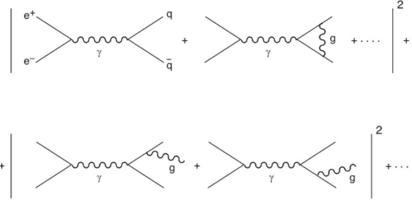
The Final State in e + e − Annihilation
Deep Inelastic Scattering

Resummation for Deep Inelastic Structure Functions
Polarized Deep Inelastic Scattering

Factorisation and the QCD Improved Parton Model

The section σ ∼ LμνWμν is given in terms of the product of a leptonic (Lμν) and a hadronic (Wμν) tensor. The evolution equations for the part densities are written in terms of kernels (the "split functions") which can be expanded in powers of the current link. This steep behavior is determined by the sharp drop in part densities at large x.

Fig. 4.9 Real and virtual diagrams relevant for the computation of R at 1-loop accuracy

Measurements of α s

α s from e + e − Colliders
α s from Deep Inelastic Scattering
Summary on α s

The range of Q2 and the precision of the data are not very sensitive to curvature for most values of x. Scaling violations of non-singlet structure functions would be ideal to determine αs because. A recent analysis of the same data leads to αs(mZ), but the theoretical error associated with the method and with the choice made for scale ambiguities is not taken into account.

Conclusion

In fact, the mass ρ or nucleon mass receives little contribution from quark masses (the case of pseudoscalar mesons is special, as they are Goldstone pseudobosons of broken chiral invariance). So it includes only a few old papers and, for most issues, some relatively recent papers where you can look for a more complete list of references. Open Access This chapter is licensed under the terms of the Creative Commons Attribution 4.0 International License (http://creativecommons.org/licenses/by/4.0/), which permits use, sharing, adaptation, distribution, and reproduction in any medium or format, as long as you credit the original author(s) and source, provide attribution to the license, and indicate a link to the Creative license.

QCD on the Lattice

Introduction and Outline

Historical Perspective
Outline

Except for a brief period of activity at the turn of the decade to simulate QCD with dynamical fermions, most projects in the 1990s were devoted to investigating damped QCD. We begin with an introduction to the basic concepts of the lattice formulation of QCD. The determinations of the fundamental parameters of QCD, namely the strong coupling constant and the quark mass, are the main focus of this paper and are presented in Section 5.5.

The Lattice Approach to QCD

Euclidean Quantization
Lattice Actions for QCD
Functional Integral and Observables
Continuum Limit, Scale Setting and Renormalization
Limitations and Systematic Effects
Simulations with Dynamical Quarks

We now turn to the problem of defining a discretized version of the Yang-Mills action. In the context of lattice QCD, this implies that the continuum limit, a→0, is reached by a suitable tuning of the bare parameters. The existence of the continuum limit in lattice QCD therefore corresponds to the existence of a second-order transition in the space of bare parameters.

Fig. 5.1 Graphical representation of the plaquette P μν (x) in the (μ, ν)-plane. The arrow between sites x + a μˆ and x denotes the link variable U μ (x)

Hadron Spectroscopy

Light Hadron Spectrum
Glueballs

In particular, condition number fluctuations can be controlled by separate and optimized processing of the low-energy part. The detailed functional form of the asymptotic behavior depends on the choice of boundary conditions. This means that the asymptotic behavior of the two-point correlation function is isolated only at large Euclidean times.

Fig. 5.5 Quenched light hadron spectrum computed in [47], compared with experiment. The statistical error and the sum of the statistical and systematic errors are indicated

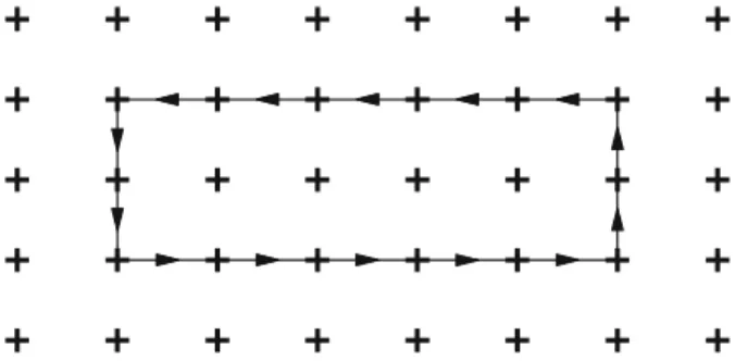
Confinement and String Breaking

In QCD with light sea quarks, the linear rise in potential cannot persist over arbitrarily large distances. Choosing to set the scale avoids the systematic uncertainty associated with extrapolating the force to an infinite distance. The diagonalization of the matrix correlator also provides information about the composition of the states in the spectral decomposition.

Fig. 5.9 Oriented product of link variables around a rectangle of area r · t

Fundamental Parameters of QCD

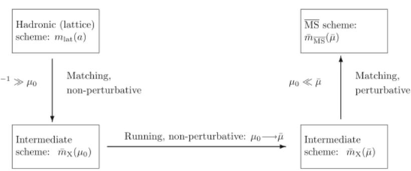
Non-perturbative Renormalization
Finite Volume Scheme: The Schrödinger Functional
Regularization-Independent Momentum Subtraction Scheme
Mean-Field Improved Perturbation Theory
The Running Coupling from the Lattice

In the above expression, the Pauli matrices act on the first two flavor components of the fields. The specific boundary conditions for the Schrödinger function ensure that the Dirac operator has a minimum eigenvalue proportional to 1/T in the massless case [73]. The results from simulations (full circles) are compared with the integration of the perturbative RG equations.