Comparative analysis of the combustion stability of diesel-methanol and diesel-ethanol in a dual-fuel engine. In the first part of this work, the simulation methodology is described in detail, where the different setups, the selected CFD models and the coupling technique between the 1D and 3D setups are discussed.
Methodology
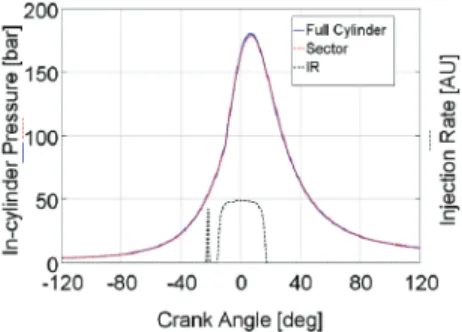
To calibrate the decay model, a constant volume vessel was reproduced in 3D-CFD software and the injection rate was simulated with a 1D injector model. Good agreement was found for the two pilot injections, but some differences were seen for the main injection.

Results and Discussion
Figure 16 presents the results obtained with constant DT (600 μs) and different ET after injection (case a vs. case b). Numerical results related to injection rate (top), heat release rate (middle), and time-varying total soot mass (bottom) of selected injection schedules are shown in Figure 18 .
Conclusions
Comparison of the effect of fuel/air interactions in a modern high speed light diesel engine. SAE Tech. Evaluation of the predictive capabilities of a combustion model for a modern common rail automotive diesel engine.SAE Tech.
Investigation on an Injection Strategy Optimization for Diesel Engines Using a One-Dimensional
Spray Model
Introduction
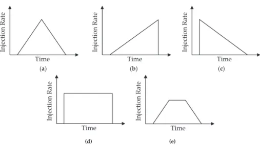
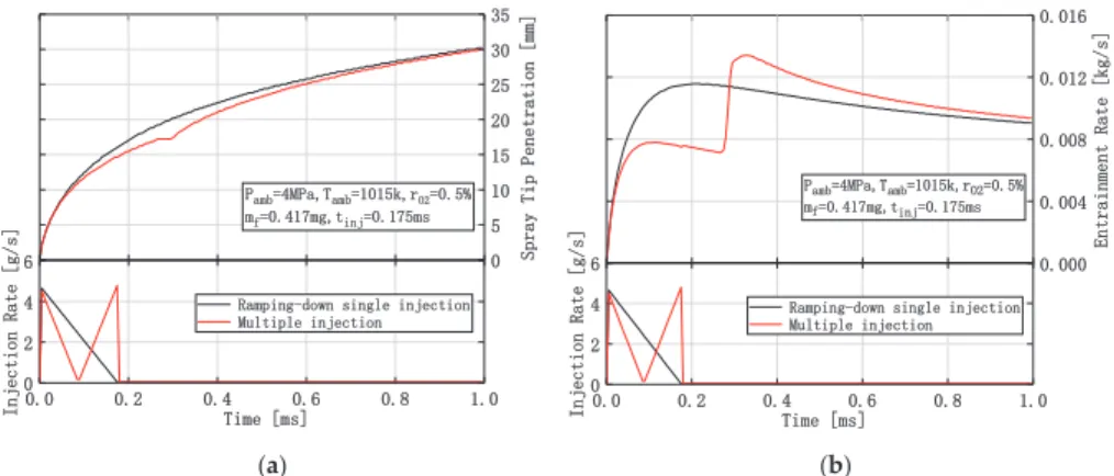
In this way, the variable injection rate design plays an increasingly important role in diesel fuel injection, which deserves an in-depth study. The result reveals that different triangular injection velocity shapes have different advantages in the spray mixing characteristic and combustion process.
Model Description 1. Spray Model
Finally, this paper also investigated the effect of the gas jet after EOI on mixture distribution and emission reduction under the decreasing injection rate shape. After that, the nozzle penetration of the multiple injection becomes smaller than that of the downward single injection due to the sharp decrease in injection rate.
A New Physics-Based Modeling Approach for a 0D Turbulence Model to Reflect the Intake Port and
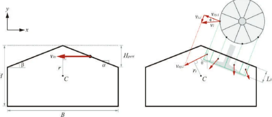
Tumble Model Development 1. Generation of Tumble Motion
In addition, these detailed flow characteristics must be properly taken into account in the tumbling calculations. Since these mass flow rates, calculated from stable CFD results (before normalization), already reflect the effect of the gate geometry.

New Turbulence Model 1. Integration into Turbulence Model
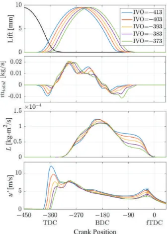
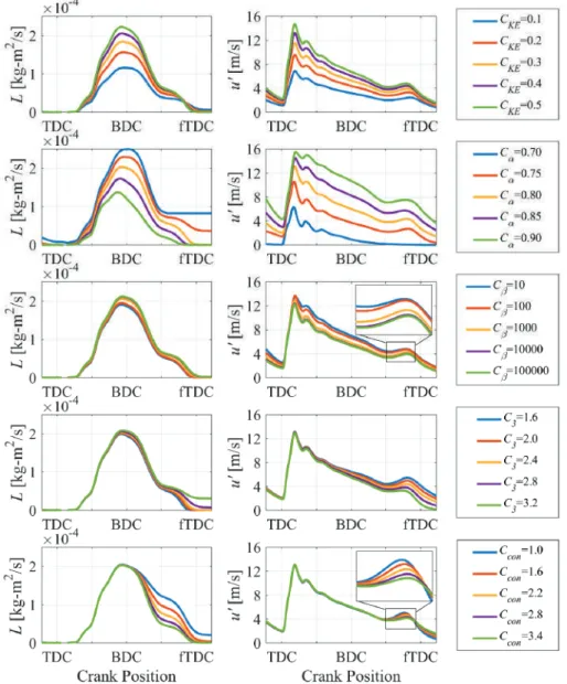
This is especially applied to the angular momentum due to the flow structure inside the cylinder. First, the effective flow velocity increases with larger CKEas derived in Equation (5), increasing the initial build-up rate of both angular momentum and turbulent intensity.
Model Validation 1. Experimental Data
The greater turbulent intensity is interpreted to increase the wrinkling of the flame sheet, i.e. the speed of flame propagation. Although not as significant as in the intake valve timing sweep, a change in laminar flame velocity is also observed.
Conclusions
An investigation of charge motion limitations and combustion duration in a spark-ignition direct injection engine. SAE Int. Observations on the Effects of Intake-Induced Swirl and Drop on Combustion Duration. SAE Trans. Predictions of downflow and in-cylinder combustion in SI engines with a quasi-dimensional model. SAE Trans.
Optimization of In-Cylinder Flow and Mixture for a Center-Spark Four-Valve Engine Using the Concept of Barrel Stratification.SAE Trans.
Comparison of Physics-Based, Semi-Empirical and Neural Network-Based Models for Model-Based
Experimental Setup and Engine Conditions
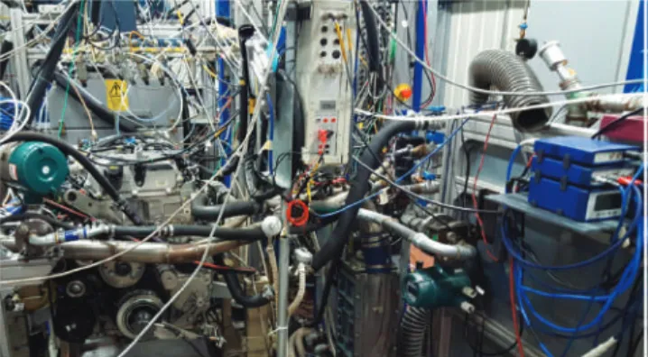
The experimental tests were performed on a Euro VI FPT F1C 3.0 L diesel engine (FPT Motorenforschung AG, Arbon, Switzerland), within a research project carried out in collaboration with FPT Industrial [11]. The activity was carried out in the dynamic test bench facility of the Politecnico di Torino. It is equipped with a VGT turbocharger, a short-cooled EGR system and a check valve on the exhaust side downstream of the turbine.
The details of the motor layout, the test rig and the sensors used (including the main accuracy) have already been described in detail in [38] and are not repeated in this paper for the sake of brevity.
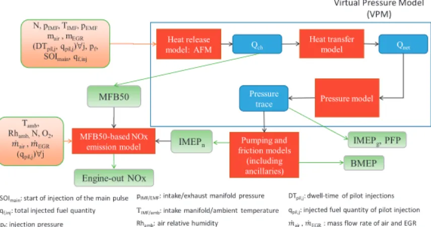
Description of the Models 1. Physics-Based Model
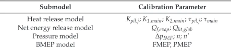
These look-up tables were obtained from the analysis of steady-state measurements. In the first step, the optimal values of all parameters are determined, test by test, based on the available experimental data. Semi-empirical models are trained on the same experimental data used to calibrate the physics-based model.
The networks are trained on the same experimental data used for the physics-based model calibration.
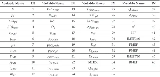
Selection of the Model Input Variables
In the second step, the partial correlation coefficient is evaluated between the dependent variables and each input variable of the initial candidate set, when the effect of the remaining input variables of the same set is removed. However, the number of parameters should not be too high, otherwise the consistency of the method will decrease. As reported in Appendix A (see Table A3), the simultaneous analysis of the Pearson and partial correlation coefficients has enabled the identification of the least and most robust correlation variables of the initial candidate set for each dependent output variable.
The remaining correlation variables in the initial candidate set, which showed intermediate values of Pearson and partial correlation coefficients, were analyzed on the basis of a sensitivity analysis to identify those to be retained and those to be excluded.
Results and Discussion
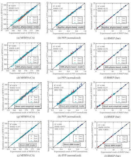
Details of the ANN parameters developed on the MATLAB platform (R2016b, MathWorks, Natick, MA, USA) are shown in Table 6. The performance of the ANNs used to directly simulate MFB50, PFP and BMEP was evaluated. The performance of the developed models was then evaluated and compared under transient operating conditions above the WHTC.
Table 9 summarizes the accuracy of the models over WHTC and under stationary operating conditions.
![Figure 4. Predicted vs. experimental values of MFB50, PFP and BMEP for the original physics-based model [12], considering the steady-state conditions.](https://thumb-ap.123doks.com/thumbv2/1libvncom/9202117.0/85.723.101.627.185.343/figure-predicted-experimental-values-original-physics-considering-conditions.webp)
Conclusions
Qht,glob global heat transfer from the load to the walls Qnet net heat output. For clarity, Figure A1 shows the temporal order of the calculation of the different variables used in the physics-based model. The generated parameters (ρSOI,TSOI), based on SOI, should be considered with higher priority than those based on SOC (ρSOC,TSOC), because of the chain of uncertainty for the estimation of SOC based on SOI;.
Comparison of the experimental and ANN fitting results for the direct estimation of MFB50 (a), PFP (b) and BMEP (c).
Implementation and Assessment of a Model-Based Controller of Torque and Nitrogen Oxide Emissions
Description of the Model-Based Controller of BMEP and NOx
The measured values PFP (peak firing pressure) and IMEPg (gross indicated mean effective pressure) are then evaluated based on the pressure in the cylinder [25]. Specifically, NOx emissions are estimated as the sum of two terms, namely the nominal NOx level emitted by the engine when operating with the baseline calibration map, and a NOx deviation term. A correction of the injection pressure pf, relative to the base value derived from the ECU maps, is also made.
It can be seen in the figure that the ETAS RP device receives the necessary input signals for the BMEP/NOx controller (i.e. the actual/state variables) from the ECU via ETK, which is an Ethernet-based communication interface.
Results and Discussion 1. Real-Time Combustion Model
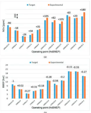
The NOx trends shown in the charts were measured by means of the engine NOx sensor. Similar to Figures 7 and 9, the time histories of the measured NOx levels (Figure 9a,c) and of SOImain (Figure 9b,d) report for the condition in which EGR is closed (Figure 9a,b) or with nominal EGR level (Figure 9c,d), considering different NOx targets. In general, the performance of the controller is very good for all the investigated tests.
Figure 14a reports the time histories of required NOx emissions (black line), measured NOx emissions (red line), and controller-estimated NOx emissions (blue line).
A Control-Oriented Engine Torque Online Estimation Approach for Gasoline Engines Based on In-Cycle
Experiment Setup
The engine has a firing order of 1-3-4-2 and all four cylinders are equipped with pressure sensors in the cylinder for the indicated torque estimate (the baseline for validation by the observer).
Engine Torque Observer Development
Validation of the indicated torque was performed in stationary and transient conditions. When the engine speed is increased to 1400 rpm (Figure 11b), the average relative error of the quoted torque estimate is within 5% of 3-6 bar. At an oil temperature of 60 °C, the maximum deviation of the friction torque is 0.75 Nm, and the average deviation is 0.53 Nm.
On the basis of the identified friction torque, the motor brake torque (Te) is decoupled from the load torque (Tload).
Numerical Investigation of 48 V Electrification Potential in Terms of Fuel Economy and Vehicle
Results
It is possible to observe that the boost pressure rises almost identically for the stoichiometric and the reference engines, while the ICE torque of the ST-Conv. In this section, the fuel consumption (although reported in terms of CO2 emissions to enable an easier comparison with legislative targets) of the investigated concepts is reported and discussed. Consequently, the activation of the electric supercharger limits the power that can be exploited by the BSG for the power split operation.
A significant reduction in fuel consumption was achieved with the Lambda-1 electrified drive system (7.3% on the WLTC and more than 15% on the RTS-95).
Impact of Electrically Assisted Turbocharger on the Intake Oxygen Concentration and Its Disturbance
Experiment Setup and Simulation Platform
This is explored based on the basics of the boosting system in this section. The compressor mass flow rate m.C can be obtained from the definition of the compressor efficiency (ηC) in [29], as shown in equations (8) and (9). HP-EGR flow deficiency when the pressure differential across the HP-EGR valve is insufficient, as illustrated by m.HP−EGR = θHP−EGRgm.HP−EGR(PTEMG,p2,m.T,T3), since PTEM is the upstream pressure of affects the EGR valve .
Another perturbation to Xoim comes from the VGT vane position, due to its influence on p3, i.e. the upstream pressure of the HP-EGR valve.
Conclusions
Xoim Oxygen concentration at the outlet of the intake manifold Xocyl Oxygen concentration in the cylinder after. A New Method of Dynamic Combustion Control Based on Oxygen Concentration Charging for Diesel Engines.SAE Tech. Control of the air system in a diesel engine using intake oxygen concentration and manifold absolute pressure with nitrogen oxide feedback.Proc.
Transient NOx Emission Reduction Using Exhaust Oxygen Concentration Based Control for a Diesel Engine.SAE Tech.
Design of an Electromagnetic Variable Valve Train with a Magnetorheological Buffer
System Overview