With a known initial condition, the differential equation can be solved for the unknown function and the solution is unique. Note that this is an approximation, because the differential equation is initially valid at all real values often.
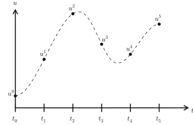
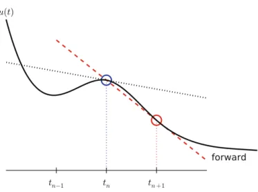
Understanding the Forward Euler Method
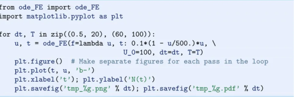
Programming the Forward Euler Scheme; the General Case Our previous program was just a flat main program tailored to a special differential
This program file, named aode_FE.py, is part of a reusable code with a general function ode_FE that can solve any differential equationbou0Df .u; t /in demo function for special case0 D0:1u,u.0/D100. This means that the call is not active if ode_FE is imported as a module in another program and the active ifode_FE.py is executed as a program.
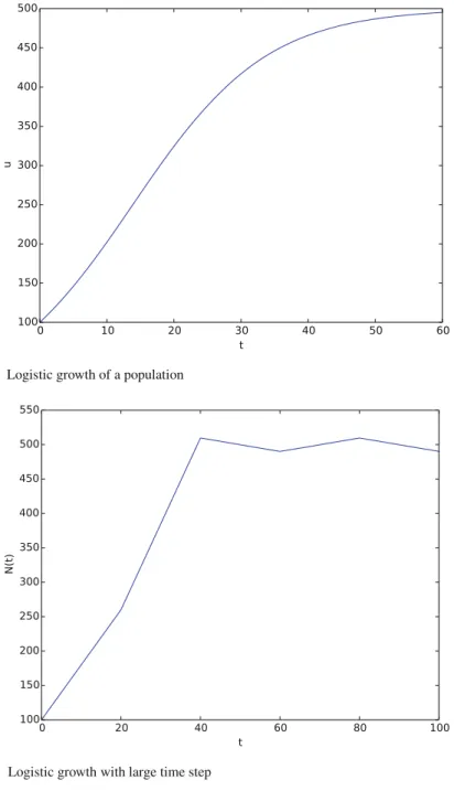
Making the Population Growth Model More Realistic
We usually call f(inode_FE) with the argument u as one array element in ode_FEfunction:u[n]. of the sum, which depends on the size of the population,N: N.tCt /N.t /Dr .N.t //N.t / : The corresponding differential equation becomes. Another option is to use the Forward Euler formula for the general problem u0Df .u; t /in usef .u; t /Dr .u/uin replace zN. The simplest choice of r .N /is a linear function that starts at some value of growth rN and decreases until the population reaches its maximum,M, given the available resources:.
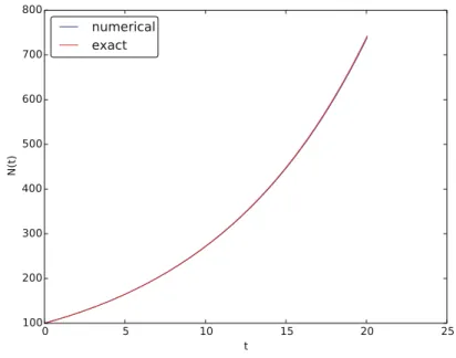
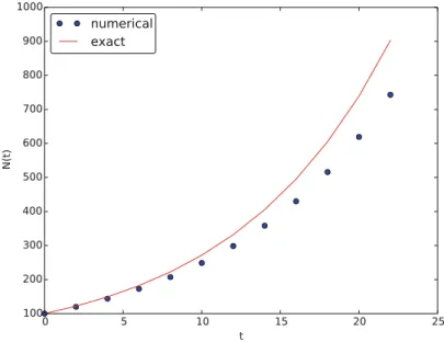
Verification: Exact Linear Solution of the Discrete Equations How can we verify that the programming of an ODE model is correct? The best
At present, world population forecasts point to growth to 9.6 billion before tapering off. Test functions should make the test successful (here success can also be a boolean expression if insert diff < tol).
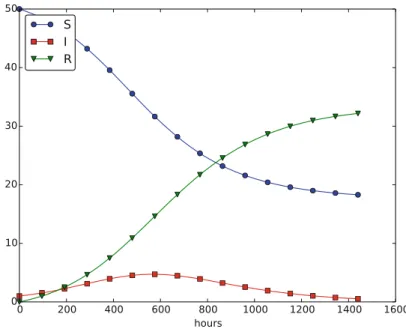
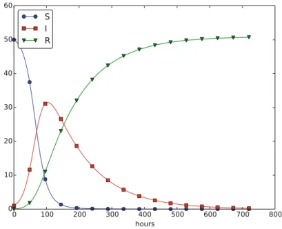
Spreading of Diseases
- Spreading of a Flu
- Programming the Numerical Method; the Special Case
- Outbreak or Not
- Abstract Problem and Notation
- Programming the Numerical Method; the General Case
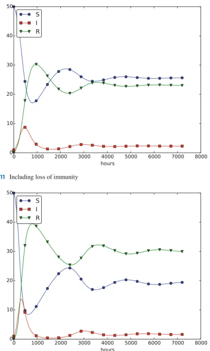
- Time-Restricted Immunity
- Incorporating Vaccination
- Discontinuous Coefficients: A Vaccination Campaign
The expected number of individuals in category S who catch the virus and become infected in the time interval t is then ptSI. Such an equation is easily determined by noting that the loss in category S is the corresponding gain in category I. Since there is no loss in category R (people are either healed and immune or dead), we are done modeling this category.
As we see, these equations are identical to the difference equations that naturally arise in the derivation of the model. It is an advantage to also write a system of differential equations in the same abstract notation. The user's f(u, t) function takes a vector u, with three components corresponding to S,I, and the Ras argument, along with the current time point[n], and must return the values of the formulas on the right-hand side of the vector ODE.
So we can write the loss in the R category astR in time, where is the typical time it takes to lose immunity.
Oscillating One-Dimensional Systems
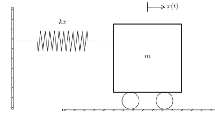
Derivation of a Simple Model
The spring is not stretched when x D0, so the force is zero, and x D0 is therefore the equilibrium position of the body. Equation (4.42) is a second-order differential equation, and therefore we need two initial conditions, one on the positionx.0/ and one on the velocityx0.0/. The solution states that such a spring-mass system oscillates back and forth as described by a cosine curve.
Numerical Solution
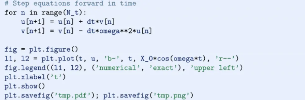
Programming the Numerical Method; the Special Case
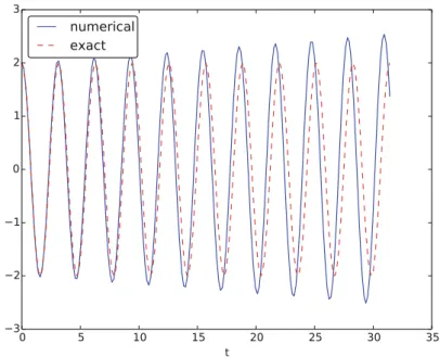
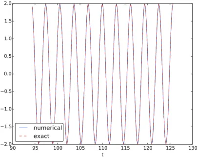
Simulate for three periods of the cosine function,T D 3P, and choose such that there are 20 intervals per period, giving DP =20 and a total ofNt DT =tintervals. Figure 4.16 shows a comparison between the numerical solution and the exact solution of the differential equation. The results are clearly better, and the best resolution gives graphs that are visually indistinguishable.
Although 2000 intervals per period of oscillation seems sufficient for an accurate numerical solution, the lower right graph in fig. . The conclusion is that the Forward Euler method has a fundamental problem with its growing amplitudes and that a very small amount is required to obtain satisfactory results.
A Magic Fix of the Numerical Method
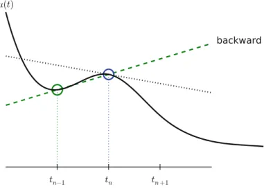
The error in the backward difference is proportional tot, the same as in the forward difference (but the proportionality constant in the error term has a different sign). In summary, using the forward difference for the first equation and the backward difference for the second equation results in a much better method than just using the forward differences in both equations. The standard way of expressing this scheme in physics is to change the order of the equations.
That is, the speed is updated first and then the positionu, using the last calculated speed. 4.50) with respect to accuracy, so the order of the original differential equations does not matter.
The 2nd-Order Runge-Kutta Method (or Heun’s Method) A very popular method for solving scalar and vector ODEs of first order is the
We see that the amplitude grows, but not as much as in the Forward Euler method. We should add that for problems where the Forward Euler method gives satisfactory approximations, such as growth/decay problems or the SIR model, the 2nd-order Runge-Kutta method or Heun's method usually performs much better and gives higher accuracy. for the same computational cost. It is therefore a very valuable method to be aware of, although it cannot compete with the Euler-Cromar scheme for oscillation problems.
Software for Solving ODEs
The derivation of the RK2/Heun scheme is also good general training in "numerical thinking". It just means that we redefine the name inside the function to mean the solution at time for the first component of the ODE system. To switch to another numerical method, just replace RK2 with the correct name of the desired method.
With all the methods in Odespy at hand, it is now easy to start exploring other methods, such as backward differences instead of the forward differences used in the Forward Euler scheme. This method is also known as ode45 because that is the name of the function that implements the method in Matlab.
The 4th-Order Runge-Kutta Method
Figure 4-23 shows a calculation example where the Runge-Kutta-Fehlberg method is clearly superior to the Euler-Cromer scheme in long-term simulations, but the comparison is not really fair because the Runge-Kutta-Fehlberg method applies about twice as many time simulations. steps in this calculation and does much more work per time step. Implementation The stages in the 4th order Runge-Kutta method can be easily implemented as a modification of theosc_Heun.pycode. Derivation The derivation of the 4th order Runge-Kutta method can be presented in a pedagogical way that brings together many fundamental elements of numerical discretization techniques and illustrates many aspects of 'numerical thinking' in constructing approximate solution methods.
Note that the 4th-order Runge-Kutta method is completely explicit, so there is never any need to solve linear or non-linear algebraic equations, no matter how it looks. The Odespy package supports many sophisticated explicit Runge-Kutta methods, but not yet implicit Runge-Kutta methods.
This is true: the numerical error actually goes as Ct4for a constantC, which means that the error approaches zero very quickly as we reduce the time step size, compared to the Forward Euler method (error), the Euler-Cromer method (error) or 2nd order Runge-Kutta or Heun's method (error2). There is a large family of implicit Runge-Kutta methods that are unconditionally stable but require solving algebraic equations involving f at each time step. Any method for a system of first-order ODEs can be used to solve foru.t /and v.t.
The Euler-Cromer method will then first use a forward difference for vnC1 and then a backward difference for vnC1. This would require a numerical method for nonlinear algebraic equations to find vnC1, while updating vnC1 by a forward difference gives an equation forvnC1 that is linear and trivial to solve by hand.
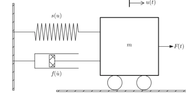
Illustration of Linear Damping
The solution of this problem corresponds to the solution of the original problem (with dimensions) with the parameters mDkDU0 D1 and bDˇ. However, the solution to the dimensionless problem is more general: if we have a solution u.N tNIˇ/, we can find the physical solution to a variety of problems since then. In this way, a time-consuming simulation can be done only once, but still provide many solutions.
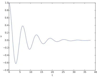
Illustration of Linear Damping with Sinusoidal Excitation We now extend the previous example to also involve some external oscillating force
Spring-Mass System with Sliding Friction
To verify that the signs in the definition of 'off' are correct, consider that the actual physical force is isf and that it is positive (i.e. f < 0) when acting against the body moving at a speedu0< 0. If no external excitation force acting on the body we have the equation of motion. The initial displacement of the body is 10 cm, and the ins.u/ parameter is set to 60 1/m.
Running the sliding friction function gives us the results in Figure 4-31 with s.u/Dk˛1tanh.˛u/(left) and the linearized versions.u/Dku(right).
A finite Difference Method; Undamped, Linear Case We shall now address numerical methods for the second-order ODE
The initial condition u0.0/D0 can help us eliminate u1- and this condition must be included somehow anyway. It turns out that this method is mathematically equivalent to the Euler-Cromer scheme. Or more precisely, the general formula (4.76) is equivalent to the Euler-Cromer formula, but the scheme for the.
Due to the equivalence of (4.76) with the Euler-Cromer scheme, the numerical results will have the same nice properties as a constant amplitude. There will be a phase error as in the Euler-Cromer scheme, but this error is effectively reduced by reducing , as already demonstrated.
A Finite Difference Method; Linear Damping
Equation (4.81) is linear in the unknown unC1, so we can easily solve for this quantity: 4.82) As in the case without damping, we have to derive a special formula for u1. The disadvantage of the backward difference compared to the centered difference (4.80) is that it reduces the accuracy in the overall scheme from t2 to . In fact, the Euler-Cromer scheme evaluates a nonlinear damping term as f .vn/ when calculating vnC1, and this is equivalent to using the backward difference above.
Consequently, the convenience of the Euler-Cromer scheme for nonlinear damping comes at a cost of lowering the overall accuracy of the scheme from second to first order int. Using the same trick in the finite difference scheme of the second order differential equation, i.e. using the posterior difference inf .u0/ makes this scheme as convenient and accurate as the Euler-Cromer scheme in the general nonlinear casemu00Cf .u0/Cs .u/DF.
Exercises
Geometric construction of the Forward Euler method
Make test functions for the Forward Euler method
Implement and evaluate Heun’s method
It is interesting to see how far off the curve the Forward Euler method is when Heun's method can be considered "exact" (for visual purposes).
Find an appropriate time step; logistic model
Find an appropriate time step; SIR model Repeat Exercise 4.4 for the SIR model
Model an adaptive vaccination campaign
Write up the complete model, implement it and repeat the case from Section 4.2.8 with various choices of parameters to illustrate various effects.
Refactor a flat program
Simulate oscillations by a general ODE solver
Compute the energy in oscillations
Use a Backward Euler scheme for population growth
Use a Crank-Nicolson scheme for population growth
Understand finite differences via Taylor series
Write down the Taylor series for u.tn/aroundtnC12t and the Taylor series for u.tnCt / aroundtnC 12t. Subtract the two series, solve with respect to u0.tnC12t /, identify the finite difference approximation and the error terms on the right, and write the leading order error term. Can you use the leading order error terms in a)-c) to explain the visual observations in the numerical experiment in Exercise 4.12?
Use a Backward Euler scheme for oscillations
Use Heun’s method for the SIR model
Use Odespy to solve a simple ODE Solve
Set up a Backward Euler scheme for oscillations
Set up a Forward Euler scheme for nonlinear and damped oscillations
Discretize an initial condition