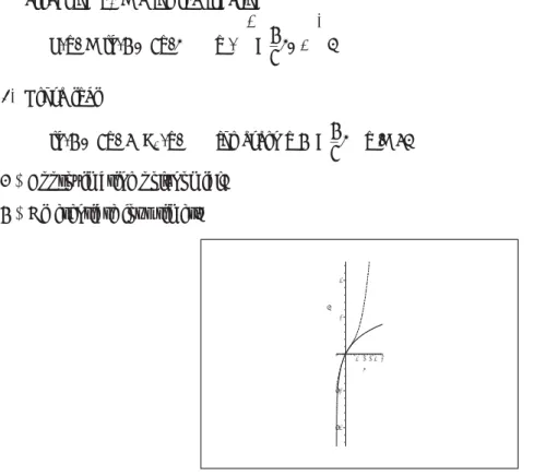
Real Functions in One Variable - Taylor's... - eBooks and textbooks from bookboon.com

Example 1.4 Set up Taylor's formula forn= 2 with the expansion point x0= 0 for the function f(x) = Arctan 2x. Example 1.8 Assume that the function f(x) is of class C∞ near the point x0∈R and that f(x0) = 0.

Figure 1: The graph of f (x) = sin x, and the tangent parallel to the x-axis, corresponding to ξ = π 2 .

2 Estimates of remainder terms

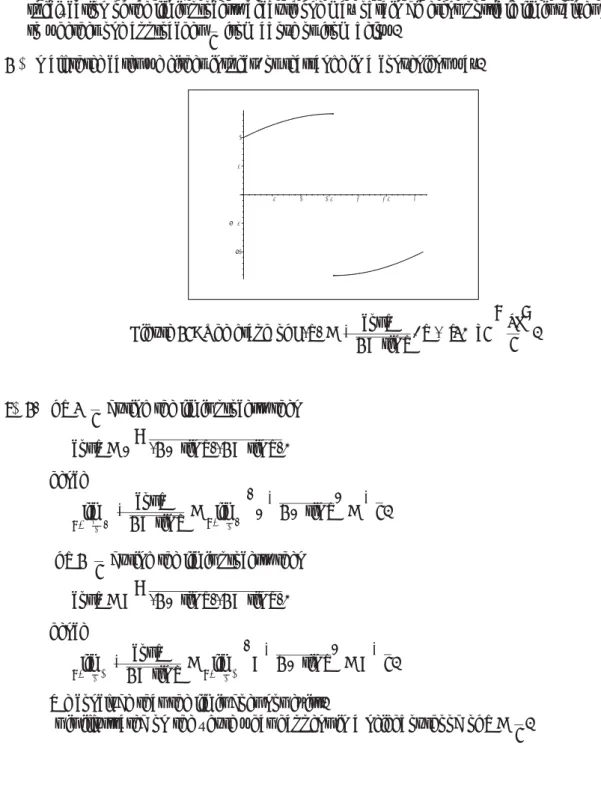
This is also the case ix2, so we get the estimate of the remaining term. Put in the Taylor polynomial and then proceed with the evaluation of the remaining term.

STUDY AT A TOP RANKED

Click on the ad to read more Click on the ad to read more Click on the ad to read more Click on the ad to read more Click on the ad to read more Click on the ad to read more.

INTERNATIONAL BUSINESS SCHOOL

Click on the ad to read more Click on the ad to read more Click on the ad to read more Click on the ad to read more Click on the ad to read more Click on the ad to read more Click on the ad to read more Click on the ad to read more. Click on the ad to read more Click on the ad to read more Click on the ad to read more Click on the ad to read more Click on the ad to read more Click on the ad to read more Click on the ad to read more Click on the ad to read more Click on the ad to read more.

CLICK HERE

By successive differentiation we get where we will use the third derivative in the evaluation of the remaining term. Click on the ad to read more. Click on the ad to read more. Click on the ad to read more. Click on the ad to read more. Click on the ad to read more. Click on the ad to read more. Click on the ad to read more. per ad for more Click on ad for more Click on ad for more Click on ad for more.

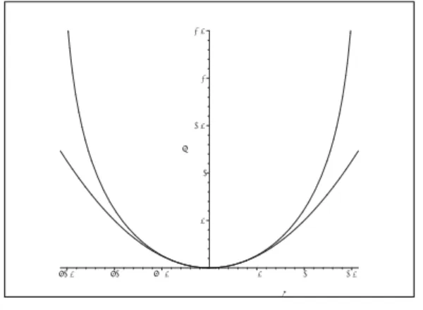
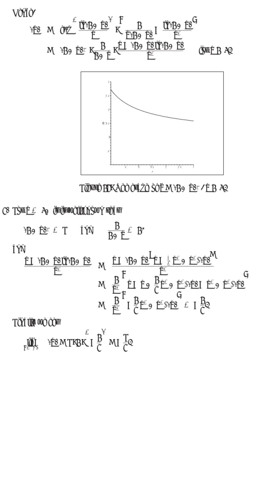
Figure 6: The graphs of f (x) = (1 + x) 2 ln(1 + x) and P 3 (x), − 0, 4 ≤ x ≤ 0, 4 with an indication of the interval [ − 0, 1; 0, 1].

3 Approximating polynomials

Click on the ad to read more Click on the ad to read more Click on the ad to read more Click on the ad to read more Click on the ad to read more Click on the ad to read more Click on ad to read more Click on ad to read more Click on ad to read more Click on ad to read more Click on ad to read more Click on ad to read more Click on ad to read more Click on the ad to read more Click on the ad to read more. Click on the ad to read more Click on the ad to read more Click on the ad to read more Click on the ad to read more Click on the ad to read more Click on the ad to read more Click on ad to read more Click on ad to read more Click on ad to read more Click on ad to read more Click on ad to read more Click on ad to read more Click on ad to read more Click on ad to read more Click on ad to read more Click on ad to read more Get help now.

Figure 9: The graph of y = ln(1 + 2x) and its approximating polynomial y = 2x − 2x 2 + 8

4 Limit processes

The order of the zero at 0 in the denominator is 1 in (1) and 2 in (2), so the numerators must be expanded similarly. Clearly, the denominator = 0 for x = 0 in (1), so since the numerator tends to −∞, it follows by inspection that (1) is divergent.

EXPERIENCE THE POWER OF FULL ENGAGEMENT…

Example 4.6 Consider the functions below for x → 0 by first placing all the terms on the same break line:. Click on the ad to read more Click on the ad to read more Click on the ad to read more Click on the ad to read more Click on the ad to read more Click on the ad to read more Click on the ad to read more on the ad to read more Click on the ad to read more Click on the ad to read more Click on the ad to read more Click on the ad to read more Click on the ad to to read more Click on the ad to read more Click on the ad to read more Click on the ad to read more Click on the ad to read more Click on the ad to read more Click on the ad to read more read Click on the ad to read more.

SETASIGNThis e-book

We will find a value of the function Bβ(λ) for λ= 0, so that the function becomes continuous at λ= 0. The purpose of the current example is partly to find the Taylor expansion, and partly to apply it in a limit process -. Therefore, we will find the Taylor expansions of the numerator and denominator of order 2.

Figure 13: The graph of y = (1 + x) x 1 , x > 0.

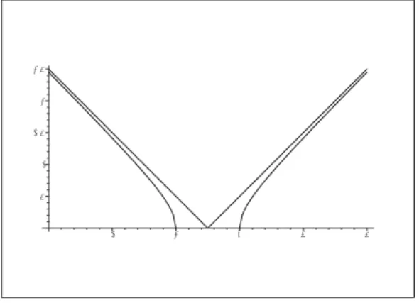
5 Asymptotes

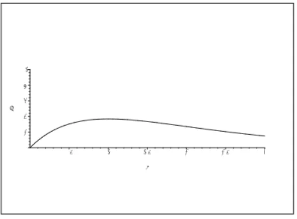
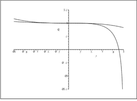
Since the function is defined continuously in the endpoints x = 2 and x = 3, we do not have asymptotes at these points, although of course we have vertical half-tangents. The function is not defined atx= 0, so there is a possibility of asymptotes forx→0, forx→+∞, and forx→.

6 Improper integrals

Click on the ad to read more. Click on the ad to read more. Click on the ad to read more. Click on the ad to read more. Click on the ad to read more. Click on the ad to read more. Click on the ad to read more. per ad to read more. Click on the ad to read more. Click on the ad to read more. Click on the ad to read more. Click on the ad to read more. Click on the ad to read more. Click on the ad to read more. Click on the ad to read more. Click on the ad to read more. Click on the ad to read more. Click on the ad to read more. Click on the ad to read more. Click on the ad to read more. Click on the ad to read more. Click on the ad to read more. Click on the ad to read more. Click on the ad to read more. Click on the ad to read more. Click on the ad to read more. Click on the ad to read more. Click on the ad to read more. Click on the ad. to read more Click on ad for more Click on ad for more Click on ad for more Click on ad for more Click on ad for more Click on ad for more Click on ad for more. Click on the ad to read more. Click on the ad to read more. Click on the ad to read more. Click on the ad to read more. Click on the ad to read more. Click on the ad to read more. Click on the ad to read more. per ad to read more. Click on the ad to read more. Click on the ad to read more. Click on the ad to read more. Click on the ad to read more. Click on the ad to read more. Click on the ad to read more. Click on the ad to read more. Click on the ad to read more. Click on the ad to read more. Click on the ad to read more. Click on the ad to read more. Click on the ad to read more. Click on the ad to read more. Click on the ad to read more. Click on the ad to read more. Click on the ad to read more. Click on the ad to read more. Click on the ad to read more. Click on the ad to read more. Click on the ad to read more. Click on the ad. for more Click on ad for more Click on ad for more Click on ad for more Click on ad for more Click on ad for more Click on ad for more Click on ad for more Click on ad to read more Click on ad for more Click on ad for more Click on ad for more Click on ad for more. Click on the ad to read more. Click on the ad to read more. Click on the ad to read more. Click on the ad to read more. Click on the ad to read more. Click on the ad to read more. Click on the ad to read more. per ad to read more. Click on the ad to read more. Click on the ad to read more. Click on the ad to read more. Click on the ad to read more. Click on the ad to read more. Click on the ad to read more. Click on the ad to read more. Click on the ad to read more. Click on the ad to read more. Click on the ad to read more. Click on the ad to read more. Click on the ad to read more. Click on the ad to read more. Click on the ad to read more. Click on the ad to read more. Click on the ad to read more. Click on the ad to read more. Click on the ad to read more. Click on the ad to read more. Click on the ad to read more. Click on the ad. for more Click on ad for more Click on ad for more Click on ad for more Click on ad for more Click on ad for more Click on ad for more Click on ad for more Click on ad for more Click on ad for more Click on ad for more Click on the ad for more Click on the ad for more Click on the ad for more.