Rydberg states of diatomic and polyatomic molecules using model potentials

RYDBERG STATES OF DIATOMIC AND POLYATOMIC MOLECULES USING MODEL POTENTIALS

Thesis by

Timothy Charles Betts

In Partial Fulfillment of the Requirements For the Degree of

U..Jctor of Philosophy

California Institute of Technology Pasadena., C2Jifornia

1972

(Submitted December 16, 1971)

i i

Acknowledgments

I wish to express my appreciation to Dr. Vincent Mc Koy for suggesting the project described in this thesis and for discus- sion and advice given throughout the course of my studies.

I would also like to thank Dr. Nicholas W. Winter for advice and assistance with various stages of programming encountered in this work.

Finally, I would like to thank my wife, Jeanette, for the encouragement and support she has given me in the preparation of this thesis.

Abstract

A simple model potential is used to calculate Rydberg series for the molecules: nitrogen, oxygen, nitric oxide, carbon monoxide, carbon dioxide, nitrogen dioxide, nitrous oxide, acety- lene, formaldehyde, formic acid, diazomethane, ketene, ethylene, allene, acetaldehyde, propyne, acrolein, dimethyl ether, 1, 3- butadiene, 2-butene, and benzene. The model potential for a molecule is taken as the sum of atomic potentials, which are calibrated to atomic data and contain no further parameters. Our results agree with experimentally measured values to within 5-10%

in all cases. The results of these calculations are applied to many unresolved problems connected with the above molecules.

Some of the more notable of these problems are the reassignment of states in carbon monoxide, the first ionization potential of

nitrogen dioxide, the interpretation of the V state in ethylene, and the mystery bands in substituted ethylenes, the identification of the R and R' series in benzene and the determination of the orbital scheme in benzene from electron impact data.

Section 1.

2.

3.

4.

4.1 4.2 4.3 4. 4 4.5 4. 6 4.7 4.8 4.9 4.10 4.11 4.12 4.13 4.14 4.15 4.16 4.17 4.18 4.19

iv

TABLE OF CONTENTS

Title Page

RYDBERG SERIES •••••••••••••••••••••••••. o • • • • • • 1 PSEUOOPOTENTIALS AND MODEL POTENTIALS.

ATOMIC CALIBRATION .•.•••••

MOLECULAR CALCULATIONS.

. ... .

15

28

Nitrogen .

• .42 .49

• • • • • • • • • • • • • • • • • • • • • • • • • • • • • • • • • • 0 • • • •

Oxygen •••••• ^{• • • • • 0} • • • • • • • • • • • • • • • • • • • • • • • • • • • 0 • • 62

• • • • • • • • • • • • • • • • • • • • • • • • • • 0 0 • •

Nitric Oxide ••••••

Carbon Monoxide. • • • • • • • • • • • • • • • • • • • 0 • • • • • • • 0 • • •

• . 73 .83

•••••o••••••••••••e•eooeo•••••

Carbon Dioxide .••

Nitrogen Dioxide. e o o o o e o e e e • • • • • • • • • o o e o o o o e o o e e

•• 93 110 Nitrous Oxide. e e e o e e e e e e e e e e e e e e e e e e o o o e e e e e e e e .122 Acetylene ••••• ••o•••oo••••••••••••••••••••••••• .135 Formaldehyde. eeoeoo••••••••••••••••o••••••••••

Formic Acid ••

.146

•••••oo••••••••••••••eeoeoooee•••• 153 Diazomethane.

Ketene ••.

O O O O e e O O O O O O O O O O O O O O O O O • e O O O O O O O O O 159

• • • • • • e o o e e e e o o e o e e o o o o o o o o e o • o • • • • • • •

Ethylene. _{••••••••o•.}•0••••••••••••••000000000000

Allene ••• 000000•••••••••••••••••••00••0••••

Acetaldehyde.

Propyne •.

••••oo•••••••••••••••••••••••o•o••

••••••&••o•••e•••••••••••••••o•••••••

Acrolein .•••••• • • • • • e • • • • • • • • • • • • • • • • • • • • • • • • • •

Dimethyl Ether • ^{• • • • 0} • • • • • • • • • • • • • • • • • • • • • • • • • • •

1, 3-Butadiene .•

166 .174 .187 .195 .200 .207 215 . 220

v

Section Title Page

4. 20 2-Butene ... 231 4. 21 Benzene ... o • • • o • • • • • • • • • • • • • • ,, • • • • • • • • • • • • 241 5. CONCLUSIONS ... ^o o • • • • • • • • • • • • • • • • • • • • • • • • • • 253

APPENDIX A. Rydberg States of Diatomic and

Polyatomic Molecules Using Model Potentials ••••.. 259 APPENDIX B. Assignments of Rydberg Series •••••••••••••• 310

1

1. RYDBERG SERIES

~

Any group of atomic or molecular states of the same spin and orbital symmetry whose term values v follow the simple formula:

(1) v

=

l.P. - R/(n - cS) ² n -_- 1 2 3· · · ' '

where I. P., R, and

o

are constants, are said to belong to a Rydberg series, and the states are called Rydberg states. In the above formula I. P. is called the ionization limit of the series, R is the Rydberg constant ^rw 109, 677. 581 cm ^{- l} (13. 595 eV) and cS is the quantum defect. In most cases the quantum defect

o

depends somewhat on the value of n, but this dependence is very slight and is usually ignored.

The above definition is a purely experimental definition and would have been discarded long ago had it not proven itself useful.

The fact that there are Rydberg series, and indeed Rydberg series are observed in practically every atom and molecule, suggests that there is some common, underlying physics behind the simple

Rydberg formula. This is indeed the case. It has been both inferred experimentally and demonstrated by calculations that Rydberg states correspond to states with an electronic configura- tion such that an electron in an orbital, the Rydberg orbital, occupies mainly a regional space exterior to the region occupied by the other electrons. These other electrons and the associated nuclei constitute the "core" about which the Rydberg electron

travels in much the same fashion as it would travel about an effective potential field derived from these electrons and nuclei.

The different members of the Rydberg series correspond to dif- ferent Rydberg orbitals of the same symmetry which occupy posi- tions more and more removed from the core potential.

The details of how this comes about for atomic sodium have been given by Slater .1

We shall give a treatment similar to Slater's here.

First we note that for sodium the Rydberg electron moves in the potential field created by the nucleus and the inner filled shells of electrons. The charge density of these filled shells is spherically symmetrical; furthermore the motion of the electrons within these shells is practically independent of the behavior of the outer electron. This means that we may replace the effect of the nucleus and the inner filled shells of electrons with a single, spherically symmetric potential field which is the same for all of the possible Rydberg states of sodium.

The analytical form of this field for sodium, Zp(r), has been given by Slater2

and is reproduced in Figure la. We note that for r greater than about 1. 5 a. u. the field becomes hydro- genic. But the energies of sodium are not the same as those for hydrogen This means that the outer part of the wavefunctions for the Rydberg orbitals correspond to the general solutions of the hydrogen radial wave equation with energies equal to the energies of the sodium atom. These solutions, which go to zero as r

approaches infinity, are valid down to r₀

=

1. 5 a. u. For values

3

II 9

Z

p(r)

0.5 1.0 1.5 2.0

r(a.u.)

Figure la. Zp(r) as a Function of r

- 0.2

Figure lb. bolutions for the Slater Potential

4

of r smaller than this, the wavefunctions of the Rydberg orbitals are solutions of the Schr6dinger equation with the sodium potential given by Slater. These solutions, which behave properly at the origin, are the be joined on to the general hydrogenic solutions at r

=

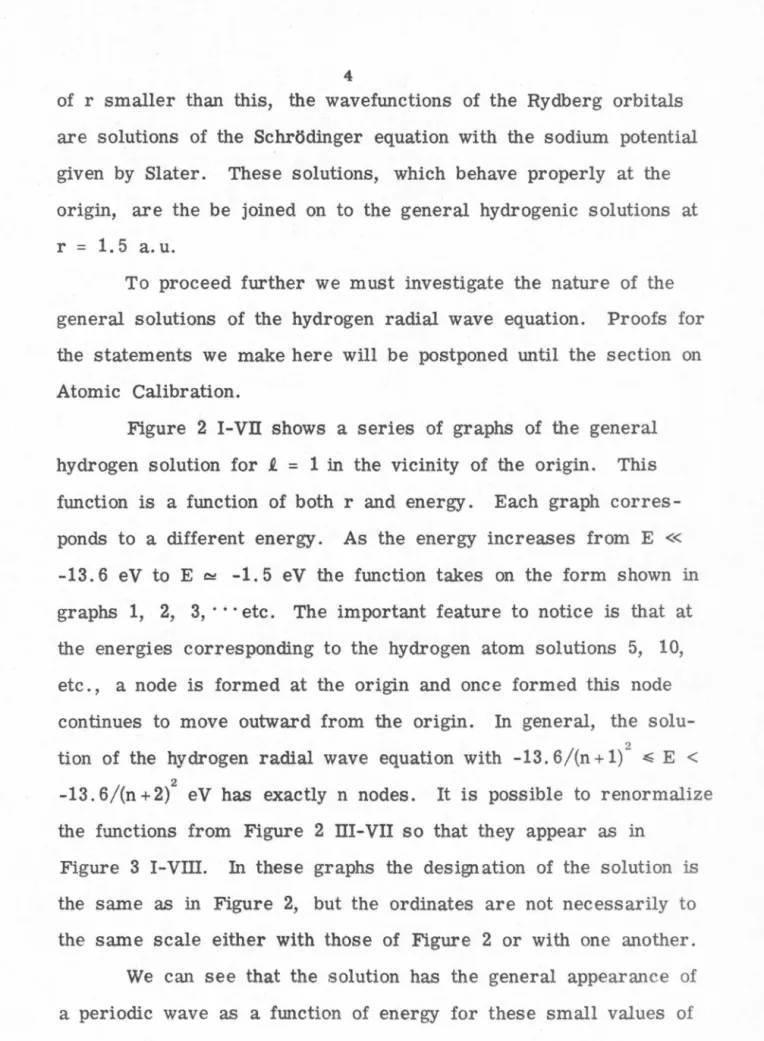
1. 5 a. u.

To proceed further we must investigate the nature of the general solutions of the hydrogen radial wave equation. Proofs for the statements we make here will be postponed until the section on Atomic Calibration.

Figure 2 I-VII shows a series of graphs of the general hydrogen solution for l.

=

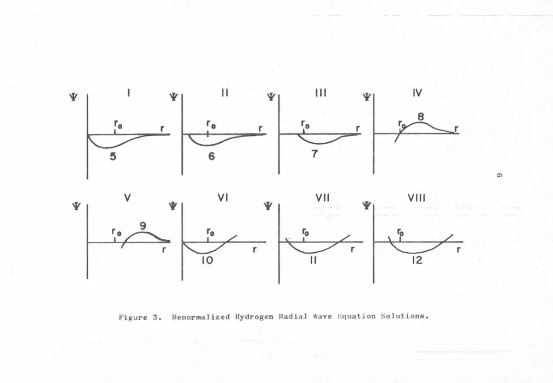
1 in the vicinity of the origin. This function is a function of both r and energy. Each graph corres- ponds to a different energy. As the energy increases from E « -13. 6 eV to E ^C!:! -1. 5 eV the function takes on the form shown in graphs 1, 2, 3, · · ·etc. The important feature to notice is that at the energies corresponding to the hydrogen atom solutions 5, 10, etc., a node is formed at the origin and once formed this node continues to move outward from the origin. In general, the solu- tion of the hydrogen radial wave equation with -13. 6/(n + 1) 2 ~ E <

-13.6/(n+2) eV has exactly n nodes. 2 It is possible to renormalize

the functions from Figure 2 III-VII so that they appear as in

Figure 3 I-VIII. In these graphs the designation of the solution is the same as in Figure 2, but the ordinates are not necessarily to the same scale either with those of Figure 2 or with one another.

We can see that the solution has the general appearance of a periodic wave as a function of energy for these small values of

F'igure 2. 8olutions of the IJydogen Radial wave l!:.quation

'i'

I

^{I 'i'}

^I

^{11 'i'}

I

^{111 'i'}

I ^IV

ro I

^ro

I

^ro

I

r 8

r

.

^{r l r} ~r

~

I

5 I ⁶ I

⁷

^I

O'l

v ., ^{VI VII}

^~

^VIII

'i' I

'f

I

:>,,., 9 l

^{'o I 7}

^L.

_r

I _~L.r

^·o

I

^{~ r}

10 II 12

Figure 3. Renormalized Hydrogen Radial Wave 1·;quation Solutions.

7

r. The period is equal to 1 in terms of the variable n, where n = ../RJE; and E is measured in Rydbergs. This being the case, we can classify the solutions of the hydrogen radial wave equation with respect to the phase

o

that this periodic wave has with some point r₀ • Setting the phase of the hydrogen atom solutions equal to zero, the energies of the solutions with phase

o

will have the

values:

(2) En

=

-R/(n - o) ² n

=

1 2 3 · · ·

' '

Finally, we note that since the solutions with phase

o

^are

all represented by essentially the same periodic wave in the region of small r, their boundary conditions are all necessarily the same too. We will find this property most useful later on.

Next, we turn to the investigation of the solution of the Schrodinger equation for the sodium atom potential. It is found that for small r's the solutions of this equation are nea_rly indepen- dent of energy for a reasonable range of energy, i.e. -5 eV < E <

0 eV. This can be seen in Figure lb, taken from Slater, 3

where the 3s and 4s functions calculated for Slater's sodium potential have been plotted for small values of r. The functions have been renormalized so as to agree as closely as possible over this range. The reason for this approximate independence of energy is that in this range of r the effective potential term of the

Schrodinger equation 2µe²Zp(r)/n\· - i(f + 1)/r² is very large numerically compared with ^- the energy eigenvalue term ⁿ .:.µEn/li ^{, 2} .

Thus small variations in En make very small relative changes in

the classical kinetic energy, and hence in the wavefunction. In more physical terms, when the electron penetrates into the interior of the atom, where Zp(r) is larger than unity, it speeds up so much on account of the nuclear attraction that its motion is almost independent of the very small amount of kinetic energy which it had when it entered the atom.

Knowing the properties of the general hydrogen solution and the solutions of the Schr6dinger equation for the sodium potential

Zp(r), we must now join these functions together at our boundary r ₀ ⁼ 1. 5 a. u. From the above, we know that all of the solutions for the sodium potential have practically identical boundary condi- tions at r₀

=

^{1. 5} a. u. since they are nearly energy independent for this range of r. Using these boundary conditions we search for the energy which corresponds to the general hydrogen solution with the same set of boundary conditions at r

=

r₀ ^• Once this energy is found, we can determine the phase of this solution, and imme- diately we know of a discrete infinity of solutions with the same boundary conditions, i.e., those solutions which have the same phase as our original solution. These other general hydrogen solu- tions must join onto the other sodium potential solutions since the boundary conditions are the same at r

=

r₀^, and we have con- structed all of the wavefunctions for the Rydberg orbitals. The energies of these Rydberg orbitals will then be:

(3) E

=

-R/(n - o) n

2 n=l 2 3···

'

'

9

We see from the arguments above that the dependence of

o

upon n is a function of how nearly alike the boundary conditions are for the general hydrogen solution with the same phase; and how energy independent the solutions of the sodium potential are. ^In practice these approximations hold to a very high degree so that

o

^{is inde-}

pendent of n to within a few percent.

Formula 3 can be made to agree with formula 1 given at the beginning of this section by noting that as n becomes large En in formula 3 approaches zero and the Rydberg orbital moves

farther from the core. In the limit the sodium atom is ionized;

hence we see that the purpose of the constant I. P. is simply to shift the energy scale to give this experimentally measured ioniza- tion potential its correct value. Thus all of the terms of equation 1 have now been accounted for.

The above arguments have given us the general form of the Rydberg formula, but they do nothing to tell us about how

o

^depends

on f. For sodium

o

is about 1. 35 for s levels, it is 0. 86 for p levels, but very small for d and f levels. It is found that the magnitude of the quantum defect

o

depends on the amount of penetration of the Rydberg orbital into the interior of the atom. If we were to plot d and f Rydberg orbitals for the region where

Zp(r) is not unity as we did for the s orbitals in Figure lb, we would find that they were very small in this region. Hence their boundary condition is that they are practically zero with zero slope at r ₀

=

1. 5 a. u. These are the same boundary conditions that the d and f functions of the hydrogen atom obey. Hence these

energy levels are practically the same as for hydrogen (i. e., quantum defect 0 ~ 0). On the other hand, the s and p Rydberg orbitals must penetrate significantly into the core where Zp(r) is not unity. The reason for this is that a Rydberg orbital with ,say, s symmetry must be orthogonal to all other orbitats with the same symmetry. This includes the core orbitals. In order to be ortho- gonal to the core orbitals, the Rydberg orbital must have signifi- cant density within the core in order for this cancellation to be possible. Thus, as a simple rule we can say that those

t

values for which there are no occupied states in the atom will have non- penetrating Rydberg orbitals, and their energies will be almost hydrogenic. As we go from these t values to the lower ones for which there are occupied states, the Rydberg orbitals become penetrating and the quantum defect 6 increases very rapidly. The same argument for penetrating and nonpenetrating orbitals holds for diatomic and polyatomic molecules as well as for atoms.

Occupied core orbitals of the same symmetry as a Rydberg orbital are sometimes called precursors of the Rydberg orbital.

While we are still considering Rydberg states of atoms we should consider the case of nonclosed shell cores. Consider the Rydberg states of beryllium with the electronic configuration

2

(ls) (2s)(np). There are two Rydberg series represented by this electronic configuration corresponding to the symmetries ³P and

1P. The quantum defects 6 for these series will be different

because of the different exchange energy contributions to the singlet and triplet states. The question arises, if we are to interpret the

11

quantum defect

o

as a phase shift as we did for the closed shell sodium core, which

o

do we use, the singlet or the triplet? The answer to this question has been given by Mulliken; 4 he says,

"The best practical (though approximate) assumption appears to be to use

o

values corresponding to averages of observed singlet and triplet energies as suitable measures of the phase shifts." In this way the effects of the exchange contributions to the singlet and triplet states roughly cancel one another out. The same sort of averaging process should be carried out when the Rydberg states of the nonclosed shell atom are doublet and quartet, triplet and quintet, etc .

We now turn to Rydberg states of diatomic and polyatomic molecules. In the same way as we joined atomic core solutions on to the solution of the hydrogen radial wave equation to produce Rydberg orbitals in the case of the sodium atom, we want to join molecular core soh.tions on to the solution of the hydrogen radial wave equation to produce Rydberg orbitals for molecules. The difference between these two cases is that the molecular core no longer has the spherical symmetry that the sodium core and the general hydrogen solutions have. However, for large enough dis- tances from the core, the core potential approaches a -e² /r hydro- genic potential, and we can expect the solutions for the core to join on smoothly to the general hydrogen solution. The major dif- ferences in the a tnmic and molecular cases arise as a consequence of the departure of the core from spherical symmetry farther in.

For atoms we can always determine the quantum defect

o

12

unambiguously by counting up the number of radial nodes, noting the energy, and using the relation between the energy and number of nodes, as was given above. For molecular problems there are strong distortions of the core solutions corresponding to a mixing of spherically symmetric solutions of different n and .t in order to produce the proper core symmetry. This mixing destroys nodes and makes it impossible to determine quantum defects

o

unambi- guously, at least for penetrating orbitals. For non-penetrating orbitals this mixing usually does not interfere with the assignment of

o.

When we cannot assign the quantum defects

o

correctly, it is frequently wiser to classify observed Rydberg states according to their effective quantum number n*,

(4) n*

=

n -

o.

This quantity has the advantage of being experimentally available.

Despite this advantage we shall always classify states according to their quantum defects

o.

One way of getting around the difficulty in determining

a,

for diatomic molecules at least, would seem to be to assign the quantum defects of the molecular orbitals on the basis of their

United Atom limits. This has been done for some molecules.

However, it has disadvantages. For instance, in nitrogen the first

pau Rydberg orbital has one more precursor in the core than the first ^prr u Rydberg orbital does. This means that the two states with practically identical forms and energies must be assigned the quantum defects 1. 71 and . 73 respectively, which surely does not

lJ3

display the close similarity which exists between these orbitals.

Another more serious difficulty arises when a Rydberg state lies somewhere between its United Atom and Separated Atom limits.

At these internuclear distances considerable mixing of different basis functions occurs and an orbital which becomes an nd?T orbital in the United Atom limit may look like an nP?T orbital in this region.

In general, the Rydberg orbitals are fairly close to their United Atom limits, but the above circumstance does arise and must be accounted for. In the following we have in general ignored the existence of precursor orbitals and have assigned our Rydberg states according to the symmetry which they display when they are plotted. In cases where this symmetry was not obvious, states were assigned to the symmetry of the Rydberg series they were a part of, according to the Rydberg formula. Rydberg states which had similar forms and energies were assigned similar quantum numbers and quantum defects regardless of the existence of pre- cursors. Thus in effect we classify our states according to their n* values, although our notation is in terms of ~.

In closing our discussion of Rydberg states we would like to consider nonclosed shell cores in molecular Rydberg states. Where as for atomic nonclosed shell cores we could get different Rydberg states with different spin symmetry, for diatomic and polyatomic molecules we can get Rydberg states with both different spin and different orbital symmetries. Consider the nitric oxide molecule. It can have Rydberg states with the electronic configuration:

(1a)² (2a)¹ (3a)² (4o°)2 (5cr)a (11r)³ (211') (nscr)

14

corresponding to both doublet and quartet ~+, ~ and IT Rydberg series. So far only the ²~+ series has been observed experimen- tally. As in the case with atomic nonclosed shell cores we con- sider the average of the quantum defects for these different Rydberg series to be comparable to the quantum defect for closed shell core molecules. When we discuss our method of calculation further, it will be seen that this average is the quantity which we calculate directly. Thus in comparing our results with experiment, we should average the experimental results over Rydberg states with the same electronic configuration.

References

~

1. J. C. Slater, Quantum Theory of Atomic Structure, Vol. I, McGraw Hill, New York, 1960, Section 9-8.

2. J.

c.

Slater, ibid.' Fig. 9-5, pg. 228.

3. J.

c.

Slater, ibid.' Fig. 9-6, pg. 231.

4. R. S. Mulliken, J. Amer. Chem. Soc. ~3183 (1964).

15

2. PSEUOOPOTENTIALS AND MODEL POTENTIALS

The pseudopotential method in its present form was intro- duced when solid state physicists1

realized that in an atom, molecule or solid there is almost complete cancellation between' the large negative potential energy V felt by a valence electron when inside the core of an atom, and its large positive kinetic energy, which is inherent in the oscillations of its wavefunction ,,, there.

'f'v

Mathematically this cancellation can be demonstrated by showing that the wave equation for the valence electron:

(1)

can be transformed into a new equation:

where V p is a nonlocal repulsive pseudopotential which cancels o'ff most of V, leaving a weak effective potential (V + V p). In equa- tion (2)

¢v

is a pseud~wavefunction which is equal to 1/Jv outside the core, but inside the core has the oscillations of

l/Jv

removed.

There are several ways to present pseudopotentials. One way would be the historical approach2 showing how the pseudo- potential idea was developed. Another would be to show how useful they can be in solving many varied and interesting problems. 3 For our purposes we prefer to work backwards. We will first prove the most general pseudopotential theorem (which is really very

simple), then we will use this as a starting point to pick out interesting special cases and to justify our procedure. This

method has the advantage of allowing us to concentrate very sharply upon the features of pseudo potentials which we will need for

Rydberg states, while keeping in the background other features which we do not need.

We start4

by calculating the eigenvalues and eigenfunctions of H + V p' where V p is defined by:

(3)

The F are completely arbitrary functions. _c The eigenfunctions and eigenvalues of H are denoted by En and l/Jn' where n

=

c or v according to whether we are considering core or valence states.

Physically speaking, we mean by core states the inner shell elec- trons of an atom or molecule and by cf>v the Rydberg orbitals.

The mathematics of the problem, however, only supposes that the eigenvalues and eigenvectors are divided into two distinct classes and does not concern itself with any differences which may exist between these classes. The eigenvalues and eigenvectors of H + V p we denote by En and cpn, again with n

- =

c or v as above, i.e.:

(4) n

=

^c or v

Consider the core states and expand cf>c in terms of the com- plete orthonormal set of functions l/Jn. Then:

17

(5) cf>c ⁼

L;

ac' l/J c' ⁺

L;

avl/Jv

c' v

Substituting equation (5) into equation (4), and using (3), we get:

(6)

L; L;

[(Ee' - Ec)oc' c" + (F , ll/J 11) ]a ^{111/J ,}

C/ C II C C C C

In the above equation the coefficient of every l/Jn must vanish identically. Looking at the coefficients of the l/Jv's we see that

,.,

unless there is some accidental degeneracy between Ee and some Ev, all of the av's

=

0, and cf>c is a linear combination of the l/Jc's.

Furthermore, since the last two terms of equation (6) must

vanish, the energy Ec will be given by the solution of the secular equation:

We shall return to this equation later. For the present we are more interested in the orbitals ¢, which correspond to our Rydberg

v orbitals.

We calculate the valence states cf> by expanding them in v

terms of the l/Jn' s also:

(8)

18

Substituting equation (8) in equation (4), and using (3), we get:

( 9)

6

2) [ ( E -

E )

6 / + ( Fe

I

l/Jc / )]{3 c / ^l/J c c c' c v · cc

This equation can be rearranged to the form:

Again in this equation the coefficient of every l/Jn must vanish

,..,

identically. Looking at the coefficient of l/Jv we see that Ev

=

Ev.

From the coefficient of l/Jv' we have

flv' =

0 unless there is some degeneracy. Thus <l>v has the form:

(11)

where the f3c 's can be determined from the nonvanishing terms of equation (10), i.e.:

This equation must have a unique solution for the unknown coeffi- cients {3 c' unless:

19

Comparing this criterion with equation (7), we can say that there is a unique solution for the coefficients f3c' unless there is some

~

accidental degeneracy between Ev and E c. Throughout 1his proof, if some degeneracy does occur, it results in a degree of arbitrari- ness in the wavefunctions which may, however, still be chosen in the form described above.

This completes the proof of the general pseudopotential theorem. In essence it states that the wave equation

can be transformed into a new wave equation:

Provided only that V p belongs to the very general class of opera- tors having the property:

where the F c are arbitrary functions. The general form of V p is that of a projection operator which projects any function <P onto the space spanned by the functions l/Jc· An interesting special case is when Fe= (Ev - Ec)lPc· Then the pseudopotential becomes:

20

This is the Phillips-Kleinman pseudopotential and is interesting because its discovery led to all of the recent work on pseudo- potentials.

If the above were all that we could do with pseudopotentials, there would not be nearly so much time and effort spent on them as there is. For in truth, the pseudopotential wave equation (15) can be just as difficult to solve, if not more so, than the original wave equation (14). To make any progress, we must inject some physics into this purely mathematical formalism. This will lead us ultimately to the subject of model potentials.

Our point of attack will be with the effective potential V + V p· This potential depends on V p' which in turn depends on the choice of functions F c. We can, if we want, vary the F c and solve the resulting pseudo-wave equations for the resulting pseudo- wavefunctions. From the definition of V p it is clear that changes in V p bring about changes in the effective potential V + V p

primarily in the region of the core. Hopefully, then, we can find a simple effective potential which has a pseudo-wavefunction with a correspondingly simple core part. We will then use this simple effective potential for problems involving its corresponding core.

Unfortunately, for smooth effective potentials the pseudo- wavefunctions turn out to have many oscillations; and for simple, smooth pseudo-wavefunctions the corresponding effective potentials are oscillatory. Abarenkov and Heine5 attribute this behavior to the fact that when using pseudopotentials we must work with the finite subspace of core eigenfunctions, rather than a complete set

21

of functions. Thus these difficulties are inherent in the method and cann.ot be gotten around within the pseudopotential formalism.

If we are willing to go outside of this formalism we can, however, make some progress. Our primary interest is in a simple, smooth pseudo-wavefunction. We then take the effective potential corresponding to this choice of pseudo-wavefunction, and approximate it with a simple smooth model potential. The model potential cannot represent all of the oscillations present in the original effective potential, but we do not care. What we desire is that the solutions of our model potential behave similarly to the solutions of the effective potential and provide a reasonable approx- imation to the pseudo-wavefunction. It is important to realize that it is not necessary to work within the pseudopotential forma- lism to define model potentials. One can develop the model potential in an exact and rigorous manner from an independent

point of view. The only absolute requirement on a pseudo or model potential is that it gives the same energy eigenstates as the real potential.

What are, then, acceptable model potentials for atoms?

Abarenkov and Heine tried several model potentials for atoms, judging their effectiveness by how good agreement they could get between a given calculated and experimental energy. Based on this study they suggested a model potential of the form:

(18)

22

where:

and

In the above, Y l.m

(e,

^¢) is a spherical harmonic function, A

1 and r₀ are constants, and

oz

^{is the effective} charge on the atomic ion.

The model potential is written as a function of the orbital quan- tum number £ because some of the valence orbitals will be pene- trating while others will be nonpenetrating, depending on their £

values. It was felt on a priori grounds that the model potential V must be very different in these different circumstances. The

m

results of our calculations and calculations similar to ours6

have shown that for Rydberg states at least, the effect of penetrating and nonpenetrating orbitals is more or less taken into account automatically, and that we may replace the Abarenkov-Heine model potential by simply its first term. Thus for atoms an acceptable model

---

potential for Rydberg states is:

(19)

V

^{ill"' (r)}

= - {A

-oz/r

r ~ r

0

r ? r

0

The above potential has three adjustable parameters, A, r₀ and

oz.

r₀ is more or less the boundary of the core region. If we expect to get reasonable results, we see from our previous

23

discussion of Rydberg states, that r₀ must be of the order of 2. 0 a. u. The parameter A must be determined by calculation and will be different for different atoms, Oz for an atomic problem is simply equal to unity. We will return to this potential in greater detail in the section on Atomic Calibration, right now we want to go on to model potentials for molecules.

For the last few paragraphs our discussion has been limited to atoms. The problem we want to solve is that for molecules.

We ask the question, what is an acceptable pseudo or model potential for a molecule? The question about pseudopotentials for molecules is still to be answered. It will probably be the subject of chemical research for many years to come. For model poten- tials, however, we can state something definite. Our work, and the work of Hazi and Rice6 shows that an acceptable model poten- tial for molecular Rydberg states is:

(20) yMolecule

=

m

E

atoms

yatom m

That is, the model potential for a molecule can be taken as the sum of the model potentials of its constituent atoms. This is a parti- cularly simple and convenient result. It suggests that we may determine the atomic model potentials independently from some atomic property, and then simply insert these atomic potentials into our molecular problem. In this way there are no adjustable parameters in the molecular problem, all of the parameters having been fixed by the atomic calculations. This avoids a proliferation of adjustable parameters in the molecular calculation.

The results to be presented here show that this is a highly successful approach. However, there is one minor difficulty. This is due to the parameter <Sz, the effective charge on the atomic ion. For an atomic calculation oz

=

1, as was stated above. In calculating a homonuclear diatomic molecule we know by symmetry that we may set oz ⁼

!

in each one of the atoms. But what is oz in a heteronuclear di.atomic? The results of our calculations show that we may take oz

= !

here also. But the problem persists for larger molecules of low symmetry. The charge distribution for these molecules can be sufficiently distorted so that a simple hypothesis about the effective charge on each atom (e.g., each atom has oz

=

1/n in a molecule containing n atoms) gives very poor results. We have met with this problem in our calculations on 2-butene, 1, 3-butadiene and acrolein. In these cases we could get some indication of the proper charge distribution from the spectroscopy of the molecule, and using these oz's the results of our calculations were quite good. Thus our approach has poten- tially one parameter, the proper charge distribution on the mole- cule. More work on larger systems may show how to get rid of this problem.

In closing this section on pseudopotentials and model poten- tials, we want to briefly discuss the kinds of solutions we expect.

In solving our problems we use a variational approach, minimizing the quantity:

(21) ^{{¢nlT +}

v

⁺

vp l</h>

(¢nl¢n)

25

The solutions ¢n where n

=

v are our Rydberg orbitals, and we expect them to be smooth, with no nodes inside the core region.

This causes no problems in the solution of equation (21). But what about the core orbitals ¢n where n

=

c? Is it possible that in solving equation (21) we will get core orbitals along with the

valence orbitals we are seeking? For a pseudopotential defined by equation (16) the answer is yes I Weeks, Hazi and Rice3 have

attempted to define a pseudopotential which does not have this some- what undesirable property, which they call variational col!apse.

But we see from our derivation of model potentials that a general definition of a pseudopotential like equation (16) is necessary if we want to make the transition to model potentials, and that variational collapse is always a possibility when working with model potentials.

The fact that core solutions can appear in our calculations at times makes some of our results a little uncertain, but most of the time it is no trouble at all.

If we are usi,ng a pseudopotential V p for which we know the functions F c' we can calculate from equation (7) where these core states lie. Thus, for instance, for the Phillips-Kleinman pseudo- potential of equation (17) we know that:

(22)

where Ev is the lowest valence state eigenvalue. Substituting this into equation (7) for the core eigenvalue Ec, we see that:

and thus that Ec = Ev for every c. Thus all of the core states are degenerate with the lowest valence state for this particular poten- tial. Further1nore, the degeneracy between E and E means that

v c

we cannot solve uniquely for· the coefficients f3 of the pseudo wave- c

function, in fact the n-fold degeneracy of the above determinant means that the f3c may be taken completely ar~itrarily, and that there are an infinity of solutions satisfying the Phillips-Kleinman pseudopotential. The general formula for this infinity of solutions is given by equation (11), where the coefficients f3 are arbitrary.

c .

It is interesting to note that this potential is the only pseudopoten- tial with such sweeping properties, and that the usual pseudo or . model potential is fairly well behaved.

In practice, in the cases of variational collapse which we have observed in our model potential calculations, the core states are usually separate and distinguishable from the valence states.

These states usually have large negative energies lying below the valence states of interest. Sometimes, however, it can be a bit difficult to decide whether or not a state is the first member of a Rydberg series or the highest core state. Whenever this happens we must use the results of calculations on similar molecules and our ¹¹feeling¹¹ of how the calculation should behave, to separate appearance from reality.

27

References

~

1. For an extensive review of this early solid state work, see W. A. Harrison, Pseudopotentials in the Theory of Metals, Benjamin, New York (1966).

2. See W. A. Harrison, ibid.

3. See J. D. Weeks, A. Hazi and S. A. Rice, Adv. in Chem. Phys.

16, 283 (1969).

~

4. This proof is taken from J. Austin, V. Heine and L. J. Sham, Phys. Rev. 127, 276 (1962).

"""""

5. I. V. Abarenkov and V. Heine, Phil. Mag. 12, 529 (1965). _{,..,_,._}

6. A. U. Hazi and S. A. Rice, J. Chem. Phys. 48, 495 (1968).

~

28

3. ATOMIC CALIBRATION

In the last section on Pseudopotentials and Model Potentials we explained how we write the model potential for a molecule as a sum of atomic potentials:

(1) ymolecule

=

M

6

atoms

yatom M

Once these atomic model potentials have been independently determined from experimental atomic data we can use them to pro- duce a parameter-free molecular nn del potential. What we want to do in this section is to calculel;te the atomic model potentials and calibrate them using experimental spectroscopic term values. In the next section on Molecular Calculations we will discuss the details of how these atomic model potentials are then used in cal- culating molecular Rydberg states.

The solution of the one-electron Schrt>dinger equation for an atomic Rydberg state with the atomic model potential

.Y~om

of the last section is straightforward, writing:

and putting

l/JE = [R~(r)/r]

^{Ytm(e, ¢)} we see, upon using the defi- nition of v~⁰m, that equation (2) splits up into two equations, namely:

(3)

d²R.£

E + [2(E - A) + .t(.£ + l)

]n.t =

⁰

dr2 r2 E

29

and

(4)

For a complete solution to our problem, we must find a solution valid in each region separately, with the property that at the point r

=

r_{0 ,} the values and the slopes of the two solutions are equal. In other words:

{R~(r)

r :::;: r₀ (5) Ri(r)

=

iii(r) r ^~ r₀ provided that at the point r

=

r₀ we have:

(6) d -£ ( )

dr fn RE r

= d~

^fn

~i(r)

The solutions of equation (3) which vanish at r

=

0 are simple rational functions in sin ../ 2

l

E _ A I r, cos ../ 2 IE - A I r, and ../ 2 IE - A I or sin h ../ 2 IE - A

I

cos h ../ 2 IE - A r, and

..f

2 IE - A I depending on whether (E - A) is positive or negative respectively. When E - A

=

0, the solution of equation (3) with these boundary conditions is simply r!+l In particular if £

=

0

sin ../2iE -Al r E-A > 0

(7)

Il~(r)

^{= r E - A}

⁼

⁰

sin h ../2 IE -Al r E - A < 0

Solutions of equation (4) are just the Coulomb functions which decay exponentially at large r. This can be expressed by the formula: ¹

where:

(9) y (n, f)

=

ⁿ²t+l r(n - t) tan (n - .e. - 1)11' r(n + f + 1)

In the above formulae r(n) is the Euler gamma function, and the functions ⁰1/-(r, E) and ¹U1(r, E) are the regular and irregular Coulomb wavefunctions. These functions, as well as the related functions:

o J.. d o_-1_

(10) D (r, E)

=

r dr U-(r, E);

i f d ^{i __}

u

D (r, E)

=

r - u-(r, E) dr

have been tabulated for f

=

0, 1, 2 over the range -1. 20 ~ E ~

-"' 0. 07 Rydbergs and 2. 0 ~ r ~ 8. 3 a. u. by Blume, Briggs and

Brooks. 2

In addition to this, Kuhn 3

has given double power series expansions for these functions which converge for small negative values of the energy. Thus we were able to determine ⁰if.(r, E),

31

1U1

(r, E), 0

n

¹(r, E) and ¹D1

(r, E) for all negative values of the energy between ^{-1. 2} ~ E ~ 0. 0 Rydbergs.

We can use equations (8) and (9) to prove our assertions about the behavior of

R~(r)/r

for small r which we made in the section on Rydberg Series to explain the creation of nodes at the origin, the interpretation of the quantum defect

o

as a phase, etc.

To do this we expand ⁰

tf

(r, E) and ¹

tf

(r, E) in power series in r, valid for small r, i.e.:

(11)

Putting these expressions into equation (4), and equating the coef- ficients of the powers of r equal to zero, we obtain:

(12) ⁰

tf

^{(r, E)}

=

.£+1 1 1 E }

const r {1 - (i+l{ + ((i+l)(.£+3) - (.£+3)]r

2 +•••

const r -i{l +

~r

+ [ E + 1 ]r2 + }

Jt. ( 4.£ - 1 )

.t (

4.£ - 1 ) • • •

It is clear that the first solution is regular at the origin, and that the second is irregular there. We note that the second solution

is not valid for i

=

0. This means that the i

=

0 solution has a higher order singularity at the origin than can be expressed by a simple nth order pole 1/rn.

Using the above expressions, we can write ~~(r)/r as:

(13)

-1

RE(r) 1 E

~ {r - _21r2 + ( )r3 + } +

~ "6"-4 •••

r

const {tan (

_

¹

~

"2 IE I

- 2)1T} {r2 1 ^{+ - + 1} _r

This function is just the un-normalized general hydrogen solution we were talking about in the Rydberg series section. It is clear that this function is infinite at the origin unless IE I

=

1/2n2, when it forms a node at the origin. The way in which the function

approaches and recedes from the coordinate axis and reflects in the abscissa at the energies IE I

=

1/2(n + ~/ is essentially determined by the factor tan (1/./ 2 IE

l -

^2)1T. The existence of the outward moving nodes is established by the principle of con- tinuity. Finally, the existence of periodic wave solutions and the phase interpretation of the quantum defect i5 is suggested by the similarity of the hydrogen atom solutions for small r, together with the principle of continuity. Using all of these simultaneously we obtain the picture of R~(r)/r, for small r, presented earlier.

Now that we have complete solutions for both R~(r) and RE(r), obeying proper boundary conditions in their respective -i

domains, we must join these functions together at the point r

=

r₀ ^•

33

This cannot be done for every value of the energy E, but only at certain discrete values En. These values will be a function of the atomic parameter A and will represent the discrete energy spec- trum En (A) for an atom with the parameter A. As we have said before, to be physically meaningful, r₀ must be approximately 2. 0 a. u. In our calculations we have taken r₀

=

2. 5 a. u. This was done so that we could compare our results directly with similar calculations by Hazi and Rice.⁴ The criterion that the functions aj(2. 5) and

R~(2.

⁵⁾ must satisfy is, according to equation (6), that their logarithmic derivatives be equal. The logarithmic derivative of R~(2. ⁵⁾ is:

(14) d - 0

dr In RE ⁼

../ 2

I

^{E - A}

I

^cot 2. 5 ../ 2

l

^{E - A}

I

1/2. 5

../ 2

I

E - A

I

c oth 2. 5 ../ 2

I

E - A

I

Similarly, the logarithmic derivative of R~(2. 5) is:

(15) ~ ^tn

R

⁰

dr E

0 0 1 0

= ! .

D (2. 5, E) + y (n, l.) D (2. 5, E) r ⁰

tf

(2. 5, E) + y (n, l.) ¹u°(2. 5, E)

E -A> 0 E - A= 0 E - A< 0

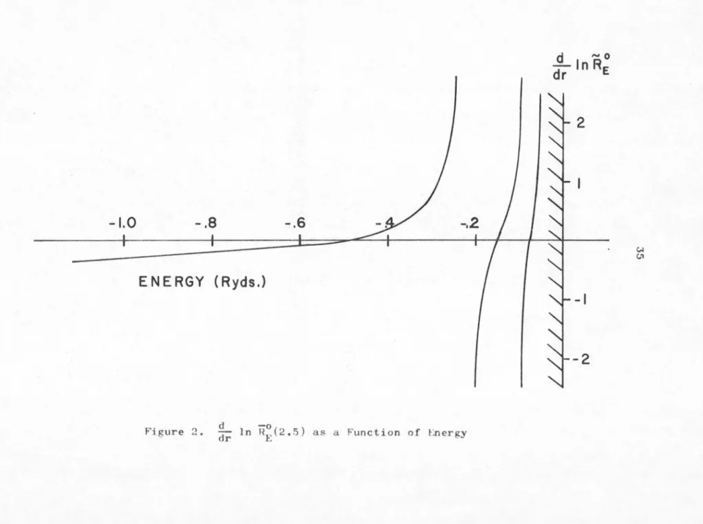
These functions are plotted as a function of energy in Figures (1) and (2) respectively. Figure (1) is fairly straightforward, the different plots on the graph representing values of A. Figure (2) however needs some explanation. The most remarkable fact about this function is the presence of infinite discontinuities. These must come about every time the energy is such that a node passes

-1.0 -.8

-.6

-.2

ENERGY ( Ryds.)

Figure 2. ~r ^In R~(2.5) as a Function of t:nergy

d ....,

⁰

dr

^In

^RE

2

-I

-2

~ C,,1

36

through the point r₀

=

2.5 a.u.

has been plotted on Figure (2).

d -o Not all of the function dr ln RE In the hatched region where IE I is small the branches of the function crowd together with a fre- quency of roughly 1/n² in the energy coordinate. This is impossible to represent on a graph.

In order to find the energy spectrlli"ll En (A), we merely have d -0

to note the places where the curve of dr ln RE for a given A inter-

d -o

sects the curve dr In RE. The energies corresponding to these intersections then form the energy spectrum En (A). Because the

d -o

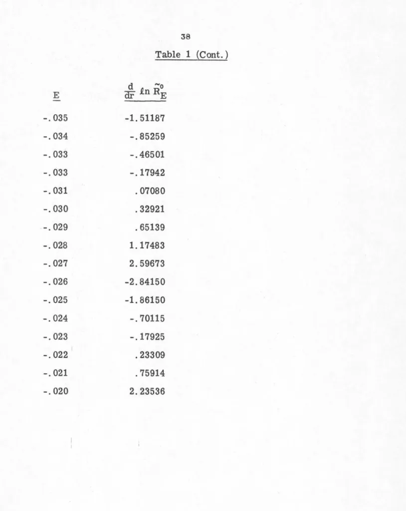
function dr ln RE has the nature of a universal function and because it is so difficult to calculate, we give a more complete tabulation of it in Table 1. One can use these results to calibrate different atomic potentials from the ones we have treated here. It is evident from looking at Figure (2) that only the part for -0. 7 ~

E Rydbergs need be considered.

In the above, we have treated in detail the case. of R~(r)

-o i

and RE(r). In principle we could use any RE(r) to determine A.

The A's determined by these different functions would then be slightly different, depending on the value of £. Lrl practice, we have restricted ourselves to £

=

0. Once we have the spectrum E (A) determined from the above functions, we compare thls cal-

n

culated spectrum with the experimentally known term values5 of the atom we wish to calibrate. By calculating En(A) for several values of A, we can interpolate to find cin acceptable value of A for the atom we wish· to represent. In Table (2) we list the

energy spectra for several values of the parameter A measured in

37

Table 1 d -o

as a function of E, for r₀ 2. 5 a. u.

dr In RE ⁼

d -o d -o

E ^dr ..e.n RE E ^dr in RE

-

-.700 -.33414 -.100 32.62618

-.600 -.21309 -.095 -3.44223

-.500 -.05653 -.090 -1. 39588

-.400 .17819 -.085 -.69546

-.350 . 36936 -. 080 -.28684

-. 300 . 71416 -.075 . 03778

-. 280 .97362 -.070 . 38012

-.260 1. 45002 -.065 . 90445

-. 240 2.76303 -.060 2.71501

-.230 5.20690 -.058 8.92571

-.220 92.99086 -.056 -6.20680

-.210 -5.23922 -.054 -2.04998

-. 200 -2.33908 -.052 -1. 05932

-.190 -1.. 37637 -.050 -.56913

-.180 -.87180 -. 048 -. 23827

-.170 -.54101 -.046 . 03902

-.150 -.06740 -.044 . 32304

-.140 .15277 -.042 .69147

-.130 .41112 -.040 1.37894

-.120 . 79442 -.038 4.69873

-.110 1. 68647 -.036 -3.18654

Table 1 (Cont.) d "'o

E

or ^tn

^RE

-

-.035 -1. 51187

-.034 -.85259

-.033 -. 46501

-.033 -.17942

-.031 . 07080

-.030 .32921

-.029 . 65139

-.028 1.17483

-.027 2.59673

-.026 -2.84150

-.025 -1.86150

-.024 -.70115

-.023 -.17925

-.022 .23309

-.021 . 75914

-.020 2.23536

39

Rydbergs. For comparison, in Table (3) we have listed the ex- perimentally observed spectra, measured in Rydbergs, for the atoms carbon, nitrogen and oxygen. This table has been con- structed using the average of the ¹P and ³P states with electronic

2 2 2

configuration (ls) (2s} (2p}(ns) for carbon, the average of the P

4 2 2 2

and P states with electronic configuration (ls} (2s} (2p} (ns) for nitrogen, and the average of the ³S and ⁵S states with electronic

2 2 3

configuration (ls) (2s) (2p} (ns) for oxygen. It will be remembered from the section on Rydberg series that this is the procedure for evaluating the term values for a non-closed shell atom.

We now only need to list the parameters which we have determined for the above atoms. Using a least squares fitting procedure we have decided on the parameters:

Acarbon c=.: • 375 a. u.

A m rogen ·t ~ . 115 a. u.

Aoxygen ~ . 045 a. u.

The above values of A are given in atomic units rather than Rydbergs because our molecular program is scaled in terms of atomic units. One fact that should be noted, is that the results of molecular calculations with these parameters show that the above values can be changed by a :factor of two or so with very little

effect upon the resulting energies.

40

Table 2

En (A), for n = 3, 4, • • •, 8, -. 50 ~ A a ~ . 75

n A= -. 50 A= -. 25 A= 0. 0 A= . 25 A=. 50 A=. 75 -

3 .54b .3694 .3091 .2846 .2717 . 2642

4 .177 .1448 .1276 .1197 .1169 .1146

5 . 088 . 0762 . 0691 .0659 . 0642 . 0632

6 . 053 . 0468 . 0433 . 0417 .0408 . 0403

7 . 035 . 0317 . 0297 .0288 .0283 . 0280

8 . 025 . 0228 . 0217 . 0210 . 021 . 021

(a) A is measured in Rydbergs

(b) The last digit in each figure is not necessarily significant.

Table 3

Experimental Spectra for

t =

0

n Carbon

- Nitrogen Oxygen

3 .2744 .2996 .3149

4 .1157 .1227 .1274

5 . 0702 . 0674 . 0690

6 . 0392 . 0425 . 0432

7 . 0280 . 0296 . 0296

8 . 0222 .0215

41

References

~

1. I. V. Abarenkov and V. Heine, Phil. Mag 12, 529 (1965).

'"'"'""

2. M. Blume, W. Briggs and H. Brooks, Tech. Rep. No. 260, Cruft Lab., Harvard University.

3. T. S. Kuhn, Quarterly of Applied Mathematics ~ 1 (1951).

4. A. Hazi and S. A. Rice, J. Chem. Phys. 48, 495 (1968).

"'"""

5. C. E. Moore, Atomic Energy Levels, National Bureau of Standards (1949).

4. MOLECULAR CALCULATIONS

In this final section we describe the general mechanics of carrying out the program which we have outlined in earlier sec- tions. We write a model potential for molecular Rydberg states v~olecule as a sum of atomic model potentials:

(1) ymolecule

=

M

L:

vatom

atom M and solve the resulting wave equation:

for the wavefunctions

ip~Yd

and corresponding energies

E~yd

of the molecular Rydberg states. Here we will limit· ourselves to general questions about coordinate systems, basis functions, etc., which apply to all of our calculations. The remaining parts of this sec- tion will discuss individually the (1) symmetries, (2) geometries, (3) spectroscopy, (4) results of calculations, (5) interpretation of the optical spectrum and (6) electron impact data for each of the molecules for which we have calculated molecular Rydberg states.

The first point which we want to take up pertains to the method of choosing coordinates. In the following sections we have always taken the z axis to be the axis of highest symmetry in the molecule, except when explicitly stated otherwise. If the molecule, or the molecule minus its hydrogen atoms, is planar, then the y axis is taken in the plane and the x axis is out of the

43

plane. Again, there may be specific exceptions to the above general rules. Distances are in atomic units ("" . 529

A),

and energy in hartree's (27.211 eV).

The general assumption used to fix the charge distribution is that an atom within a molecule containing n atoms has an effec- tive charge of

oz =

1/n. It is found that this assumptions works very well for both homonuclear and heteronuclear diatomics and triatomic molecules. For some of the larger molecules this

assumption had to be altered. Specific details will be found in the sections describing the molecules individually.

In all cases the hydrogen atoms belonging to the molecule were disregarded. Besides the fact this assumption gave good results for all of the cases considered, it was tested specifically for ethylene. For ethylene the hydrogens were included using a model potential with A

=

0. 0 and Oz

=

0. 04 at each of the hydrogen positions. Calculations on the nsa g series with this molecular potential gave:

E3s

=

3. 35, E4s

=

1. 48, E 5s

=

.83 atomic units, in comparison to:

·,

E3s

=

3. 42, E4s

=

^{1. 49,} _{E 5}^s

=

.84

for the calculation neglecting the hydrogens. It is interesting to compare this difference with the difference caused by a change in the atomic parameters for the carbon atoms themselves. A