sensors

sensors

Article

Laboratory Calibration and Field Validation of Soil Water Content and Salinity Measurements Using the 5TE Sensor

Nessrine Zemni^1,2,*, Fethi Bouksila¹, Magnus Persson³, Fairouz Slama², Ronny Berndtsson^3,4 and Rachida Bouhlila²

1 National Institute for Research in Rural Engineering, Water, and Forestry, Box 10, Ariana 2080, Tunisia;

bouksila.fethi@iresa.agrinet.tn

2 Laboratory of Modelling in Hydraulics and Environment, National Engineering School of Tunis, University of Tunis El Manar (ENIT), Box 37, Le Belvédère Tunis 1002, Tunisia; fairouz.slama@enit.utm.tn (F.S.);

rachida.bouhlila@enit.utm.tn (R.B.)

3 Department of Water Resources Engineering, Lund University, Box 118, SE-221 00 Lund, Sweden;

magnus.persson@tvrl.lth.se (M.P.); ronny.berndtsson@tvrl.lth.se (R.B.)

4 Centre for Middle Eastern Studies, Lund University, Box 201, SE-221 00 Lund, Sweden

* Correspondence: nessrine.zemni@enit.utm.tn; Tel.:+216-28-083-156

Received: 8 October 2019; Accepted: 27 November 2019; Published: 29 November 2019

Abstract: Capacitance sensors are widely used in agriculture for irrigation and soil management purposes. However, their use under saline conditions is a major challenge, especially for sensors operating with low frequency. Their dielectric readings are often biased by high soil electrical conductivity. New calculation approaches for soil water content (θ) and pore water electrical conductivity (ECp), in which apparent soil electrical conductivity (ECa) is included, have been suggested in recent research. However, these methods have neither been tested with low-cost capacitance probes such as the 5TE (70 MHz, Decagon Devices, Pullman, WA, USA) nor for field conditions. Thus, it is important to determine the performance of these approaches and to test the application range using the 5TE sensor for irrigated soils. For this purpose, sandy soil was collected from the Jemna oasis in southern Tunisia and four 5TE sensors were installed in the field at four soil depths. Measurements of apparent dielectric permittivity (Ka), ECa, and soil temperature were taken under different electrical conductivity of soil moisture solutions. Results show that, under field conditions, 5TE accuracy forθestimation increased when considering the ECa effect. Field calibrated models gave betterθestimation (root mean square error (RMSE)=0.03 m³m⁻³) as compared to laboratory experiments (RMSE=0.06 m³m⁻³). For ECp prediction, two corrections of the Hilhorst model were investigated. The first approach, which considers the ECa effect on K’ reading, failed to improve the Hilhorst model for ECp>3 dS m⁻¹for both laboratory and field conditions. However, the second approach, which considers the effect of ECa on the soil parameter K0, increased the performance of the Hilhorst model and gave accurate measurements of ECp using the 5TE sensor for irrigated soil.

Keywords:soil salinity; soil water content; FDR sensor; soil pore water electrical conductivity; sensor calibration and validation; real time monitoring

1. Introduction

In arid and semiarid countries, such as Tunisia, irrigation is necessary for improved agricultural production. Water resources with good quality are limited, resulting in the use of low-quality irrigation water. This can induce soil salinization, leading to crop yield reduction, decreasing the agricultural productivity, and causing general income loss [1,2]. Thus, accurate monitoring of soil salinity in time

and space is of great importance for precision irrigation scheduling to save water and avoid soil degradation. Over the last decades, soil dielectric sensors have been developed to measure apparent electrical conductivity (ECa) from which real soil salinity, the soil pore electrical conductivity (ECp), can be estimated [3]. Time domain reflectometry (TDR) has been established as the most accurate dielectric technique to estimate both volumetric water content (θ) and ECp in soils providing automatic, simultaneous, and continuous readings [4]. The efficiency of the TDR method has led to development of other techniques based on similar principles, such as capacitance methods. Some examples are the WET (Delta-T Devices Ltd., Cambridge, UK) and the 5TE (Decagon Devices Inc., Pullman, WA, USA) sensors, both based on frequency domain reflectometry (FDR). Compared to TDR, FDR sensors use a fixed frequency wave instead of a broad-band signal that makes them cheaper and smaller [5].

Dielectric methods are based on determination of apparent soil electrical conductivity (ECa) and soil apparent dielectric permittivity (Ka) [6]. Many models for the relationships between Ka and θ[4,7], ECa-θ, and ECa-ECp-Ka have been proposed in recent research [3,8–10]. However, dielectric properties are affected by physical and chemical soil properties. For example, high ECa affects the wave propagation, leading to errors in the estimation of Ka [11,12]. Thus, it is important to improveθ and ECp prediction models.

Hilhorst [8] presented a theoretical model describing a linear relationship between ECa and Ka to predict ECp. This linear model can be used in a wide range of soil types without soil-specific calibration. Persson [13] evaluated the Hilhorst model using TDR in three sandy soils and confirmed the accuracy of the linear model with significant dependency on soil type. Many researchers [14–17]

have tested the Hilhorst model using the WET sensor and showed that it can be improved with soil specific calibration. Using the WET sensor, improved correction of the Hilhorst model was proposed by Bouksila et al. [18], using loamy sand soil with about 65% gypsum. They found that the accuracy of ECp prediction is very poor when using standard soil parameters (K₀). Thus, they proposed a correction by introducing a third-order polynomial fitted to the K0–ECa relationship instead of using the default K0. Kargas et al. [6] introduced a linear permittivity corrected model, proposed by Robinson et al. [5], in the Hilhorst relationship. They found that the correction depends on soil characteristics and that it is valid for ECa close to 2 dS m⁻¹. These approaches consider the ECa effect on the prediction of ECp. However, research has not been performed using simultaneous controlled laboratory and field-scale experiments where effects of heterogeneity, root density, insect burrowing, etc., affect the observations [19]. Ideally, sensor calibration should be performed in structured soils due to its importance for pore size distribution and associated matrix potential [20]. Research has shown that calibration in repacked soil columns differs from calibration in disturbed soil used in laboratory experiments [21]. In addition, intrinsic soil factors such as soil temperature, presence of gravel, and microorganisms affect the soil structure and porosity contributing to the variability in ECa and Ka measurements under field conditions as compared to measurements in the laboratory [19].

Nowadays, farmers are embracing precision agriculture using sensors with high accuracy and low cost to increase yields and maintain the sustainability of irrigated land. The 5TE dielectric soil sensor, which also uses the Hilhorst model for ECp estimation, was introduced in 2007 and it is much cheaper than the WET sensor [22]. Several recent studies have investigated the 5TE probe in agricultural applications [2,23,24]. The 5TE sensor has electrodes at the end of the probe that are influenced by soil density making them sensitive to any variation in soil structure andθcontent [25]. Despite this fact, most studies on the 5TE sensor performance [16,26,27] have been carried out under laboratory conditions. Thus, almost no research has been done in the field for testing its performance for ECp estimation, neither with the most used linear Hilhorst model nor with the more recent ECp approach proposed in literature. Another important practical aspect is to determine the application range of these sensors for irrigated soils under saline conditions. For example, it is important to determine at what ECa threshold the dielectric losses are no longer negligible and need to be corrected for. Furthermore, there is a lack of understanding of how laboratory calibration can be translated into field conditions.

Thus, the sensors must be calibrated and validated under both conditions in order to assess the errors associated with translating one to the other [28].

In view of the above, the objective of the present study was to assess the performance of the 5TE sensor to estimate soil water content and soil pore electrical conductivity for a representative sandy soil used for cultivation of date palms. Both standard models and a novel approach using corrected models to compensate for high electrical conductivity were used. Results from both field and laboratory experiments were compared. The location of the field experiments was the Jemna oasis, southern Tunisia.

2. Materials and Methods

Soil parameter acronyms, data source, sensor specification and models used in the present work were presented in AppendixA.

2.1. Theoretical Considerations

Any porous medium, such as soils, can be characterized by its permittivity, which is a complex quantity (K) composed of a real part (K’) describing energy storage, and an imaginary part (K”) describing energy loss:

K=K−j K with j= √ −1 (1)

For soils with low salinity, it is often assumed that the polarization and conductivity effects can be neglected [4]. Under such conditions, the effect of K” is eliminated and K’ becomes equal to K, represented by Ka as the apparent dielectric constant [4]. Under saline conditions, the imaginary part of the dielectric permittivity increases with ECa, leading to error in the permittivity measurement. This problem becomes important for frequencies lower than 200 MHz [6]. According to Campbell [29], for a frequency range of 1–50 MHz, conductivity is the most important mechanism related to energy loss.

However, using the hydra impedance probe, Kelleners and Verma [30] found that, in general, the total energy loss is related to relaxation loss except for fine sandy soil, where it is equal to zero at 50 MHz.

2.1.1. Permittivity-Corrected Linear Model

Many researchers [5,17,31,32] have studied how well low-frequency capacitance sensors measure Ka and to what degree it is affected by K”. In general, it has been shown that the most important factor to consider is the conductivity effect on Ka, whereas the effect of relaxation losses appears to be small [4,6]. Thus, it is possible to correct the Ka reading by introducing a term for the ECa effect. Based on the work of Whalley [32], Robinson et al. [5] proposed a permittivity-corrected linear model where the theoretical permittivity can be considered equivalent to the refractive index of measurements by the TDR. Robinson et al. [5] conducted experiments using TDR and capacitance dielectric sensor in sandy soils with high ECa levels (up to 2.5 dS m⁻¹) and they proposed a linear model that includes the ECa effect on the Ka prediction according to:

√K=√

Ka−0.628 ECa (2)

From this equation, we notice that the increase of ECa (dS m⁻¹) leads to an increase in Ka. Using Equation (2), a corrected permittivity K’ can be determined eliminating the ECa effect [6].

2.1.2. Water Content Model

The dielectric constant is about 80 for water (at 20^◦C), 2 to 5 for dry soil, and 1 for air. Therefore, Ka is highly dependent onθ. Various equations for the Ka vs.θrelationship have been published. The

most usedθ-model is a third-order polynomial [4]. However, Ledieu et al. [7] showed that there is a simpler linear relationship for theθprediction with only two empirical parameters, of the form:

θ=a√

Ka+b (3)

where a and b are fitting parameters.

Figure1shows a schematic of calibration and validation possibilities forθestimations that were used in the present study. The calibration consisted of fitting of parameters in different models (Figure1). Optimal values for a and b, vs. a’ and b’ were determined by linear regression in the relationship√

Ka-θmdenoted as the CAL-Ka model (Figure1, Step-A.1) and√

K’-θmdenoted as CAL-Kar model (Figure1, Step-A.2), respectively. Theθmwas measured in experiments for different salinity levels. The standard Ledieu et al. [7] model (Figure1) was used for comparison purposes as it is the simplest known model for mineral soil. The different steps (A.1 and A.2) were first completed using laboratory experiments (laboratory calibration) and then using field data (field calibration).

The laboratory and field calibrated models were then compared with each other (Figure1, Step-A.3).

Finally, we used field data (step B.1, B.2, and B.3) to validate the laboratory experiments (laboratory model validation).

Figure 1.Schematic ofθcalibration and validation possibilities investigated in the present study.

2.1.3. Pore Water Electrical Conductivity Model

Different studies [33,34] have shown that ECa depends on bothθand ECp. Malicki et al. [35] and Malicki and Walczak [9] found that for Ka>6 and when ECp is constant, the relationship between Ka and ECa is linear. An empirical ECp–ECa–Ka model has, thus, been proposed. Based on their results, Hilhorst [8] presented the following equation applicable whenθ≥0.10 m³m⁻³:

ECp= Kw

(Ka−K0)

×ECa (4)

where Kwis the dielectric constant of the pore water (equal to 80.3) and K0is a soil parameter equal to Ka when ECa=0 (see [8], for details). According to Hilhorst [8], the K0parameter depends on soil texture but is independent of ECa. He found the range of K₀to be between 1.9 and 7.6. For best results, this should be determined experimentally for each soil type. For most soils, a value of 4.1 has been recommended. One should notice, that in the Hilhorst model (Equation (4)), the Ka, Kw, and K₀ represent the real part of the dielectric constant only. From the linear relationship ECp=f (ECa), the slope that is inversely proportional to ECp and intercept K0can be determined.

In the present study, the Hilhorst model (Figure2, Step-C.1) was tested using varying K₀soil parameters (4.1, 6 and 3.3). The K0=4.1 is the default value recommended by Hilhorst, K0=6 is the recommended value in the 5TE manual [36] while K0=3.3 is the value measured with distilled water according to the WET sensor manual [37].

Figure 2.Schematic of electrical conductivity (ECp) calibration and validation used in the present paper.

Inspired by Bouksila et al. [18] and Kargas et al. [6], a modification of the Hilhorst model was investigated. Accordingly, a permittivity-corrected linear equation (Equation (2)) can be introduced in the Hilhorst model (Figure2, Step-C.2) and ECp is predicted with two different K0values (K0=4.1 and K₀=3.3). Beside this, the soil fit parameter K₀is calculated for each salinity level by minimizing the mean square error (MSE) of the estimated ECp in the Hilhorst model (Step-C.3.1). The best fit K0

parameters are then plotted against ECa for the seven different ECp and a third-order polynomial function is determined (Step-C.3.2), and introduced in the Hilhorst model (Step-C.3). Finally, we used field data (step D.1, D.2, and D.3) to validate the laboratory experiments (laboratory model validation).

The temperature is an important factor influencing the electrical conductivity measurements;

indeed, all ECa reading were adjusted in the present work using Equation (5). Besides, during experiments the temperature effect on Kw parameter was considered using the recommended temperature correction equation in the 5TE manual [36].

ECa25=ECa[1−((T−25)× 0.02)] (5)

Measured Ka, ECa, and T in laboratory and field experiments are converted to ECp using the Hilhorst [8] model (Step-C.1), Kargas et al. [6] approach (Step-C.2), and Bouksila et al. [18] approach (Step-C.3), denoted as H, MHK, and MHB, respectively.

The different approaches in Figures1and2have not been tested before using the 5TE sensor.

The approaches CAL-Kar, MHK and MHB have previously only been tested once under controlled laboratory condition using the WET sensor. The novelty of the present work is to validate these approaches under field condition using the low cost capacitance sensor 5TE. In addition, the MHB approach developed by Bouksila et al. [18], used an experimentally determined K₀=f (ECa) relationship.

Our new approach instead uses a K0derived from best-fit parameter for each ECp level, which make the application of MHB approach much easier since there is no need for the K₀laboratory experiment.

Model performance forθand ECp, was evaluated using both the root mean square error (RMSE) and coefficient of determination (R²). In addition, mean relative error (MRE) and coefficient of variation (CV) were used for ECp andθ, respectively.

2.2. Study Area

The field study was conducted in the Jemna oasis (33^◦36’15.”N, 9^◦00’39.”E), belonging to the Agricultural Extension and Training Agency (AVFA) located in the Kebeli Governorate, southern Tunisia. The oasis is equipped with a micro-irrigation system. The main crop is adult date-palm trees. The climate is arid with an annual rainfall of less than 100 mm, which is insufficient to sustain agriculture. The annual potential evapotranspiration is about 2000 mm [38]. Groundwater, situated at 17 m soil depth, with an electrical conductivity (ECiw) of about 3.5 dS m⁻¹, is used for irrigation. The pH of groundwater is 7.8 and the geochemical facies is sodium chloride. Soil samples were collected from the top soil at 0–0.5 m depth. The soil was leached with distilled water in order to remove soluble salts and oven dried (105^◦C) for 24 h. Then, the soil was passed through a 2 mm sieve. Soil particle size distribution was determined using the sedimentation method (pipette and hydrometer) and the electrical conductivity of saturated soil paste extract (ECe) was measured according to the United States Department of Agriculture (USDA) [39]. A summary of soil properties is presented in Table1.

Table 1.Particle size percentage, pH and electrical conductivity of saturated soil paste extract (ECe) of investigated soil samples.

Depth (m) Clay (%) Fine Silt (%)

Coarse Silt (%)

Fine Sand (%)

Coarse

Sand (%) pH ECe

(dS m⁻¹)

0–0.5 5 3 4 22 65 8.5 1.8

2.3. Laboratory Experiments

Seven NaCl solutions with different electrical conductivity (0.02, 0.2, 0.5, 3.6, 5.3, 7.2, and 8.2 dS m⁻¹) were prepared for the infiltration experiments. The soil was initially mixed with a small amount (about 0.05 m³m⁻³) of the same water as used in the infiltration experiments to prevent water repellency. The soil was repacked into a plexiglas soil columns, 0.12 m in diameter and 0.15 m long (Soil Measurement System, Tucson, Arizona), to the average dry bulk density encountered in the field (about 1450 kg m⁻³).

The 5TE sensor was used for observations [23]. It is a multifunctional sensor measuring Ka, ECa, and T (for more details, see AppendixA). The measuring frequency is 70 MHz and it is a three-rod type sensor with 0.052 m long prongs and 0.01 m spacing between adjacent prongs [23,40]. The 5TE probe was inserted vertically in the center of the column. Upward infiltration experiments were carried out by stepwise pumping a known volume of a NaCl solution (45 mL) with a precise syringe pump from the bottom of the column. Twenty minutes after each injection, three measurements of Ka, ECa, and temperature were taken and averaged. This procedure was repeated until saturation (0.40 m³m⁻³) was reached. Four hours after reaching saturation, measurements were again taken and pore water was extracted from the bottom of the column with a manual vacuum pump. Electrical conductivity of extracted pore water ECpmwas measured with a conductivity meter. In total, seven upward infiltration experiments were conducted, one for every NaCl solution.

2.4. Field Measurements

Four 5TE sensors were installed between date-palm trees at four soil depths (0.10, 0.15, 0.30, and 0.45 m). The 5TE probes were connected to a Decagon Em50 data logger. The DataTrac3 software version 3.15 [23] was used to download collected data from the Em50. Volumetric soil water content and pore electrical conductivity were estimated using standard parameters of the Ledieu et al. [7] and Hilhorst [8] models, respectively. In addition, soil samples were taken by hand auger at the same depth of sensor installation on 24 April and 3 October 2018. Gravimetric water contentθmand electrical conductivity of saturated soil paste extract (ECe) were measured in laboratory according to USDA standards. The soil dry bulk density (Bd) was measured in the field using the cylinder method at five soil depths (0.1 m depth intervals to 0.5 m). During April 2018, the average soil Bd was equal to 1.43 g cm⁻³and varied from 1.3 to 1.6 g cm⁻³.

3. Results

3.1. Soil Water Content

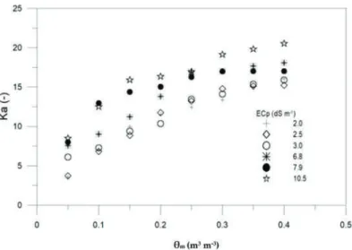
Figure3presents the relationship between Ka and observedθmwith different salinity levels (ECp, dS m⁻¹) measured during the upward infiltration experiments. For largest ECp, ECa did not exceed 2.5 dS m⁻¹. It is seen that ECa considerably affects the Ka readings, especially for high ECp. This can lead to significant errors for both Ka and ECa, indicating that 5TE probe readings need to be corrected when used in saline soils. The overestimation of Ka as ECa increases has been described by several authors (e.g., [19,27]).

In Figure4, Ka and K’ (corrected with Equation (2)) for two ECp levels (3 and 9.8 dS m⁻¹) are plotted against measuredθm. K’ values are very close to Ka when ECp≤3 dS m⁻¹, especially at lowθ (θ≤0.15 m³m⁻³and ECa≤0.43 dS m⁻¹). However, for ECp=9.8 dS m⁻¹, the difference between Ka and K’ is more pronounced, especially forθ≥0.15 m³m⁻³and ECa≥0.75 dS m⁻¹.

Figure 3.Apparent dielectric permittivity (Ka) vs. measured volumetric water content (θm) for various pore electrical conductivity (ECp) levels (dS m⁻¹).

Figure 4. Relationship Ka-θm(open circles) and K’-θm(filled circles) using the 5TE sensor for ECp=3 dS m⁻¹(a) and ECp=9.8 dS m⁻¹(b).

The calibrated parameters using laboratory data for CAL-Ka and CAL-Kar approaches are presented in Table2. For all models tested under laboratory conditions, RMSE increased with ECp. Soil water content from CAL-Kar approach matched well measuredθmfor ECp≤3 dS m⁻¹ (ECa<0.7 dS m⁻¹) and gave the bestθestimation compared to the Ledieu et al. [13] model and the soil-specific calibration CAL-Ka. However, for ECp≥6.8 dS m⁻¹, the CAL-Ka approach gave lower RMSE compared to the CAL-Kar model. For high ECp (≥6.8 dS m⁻¹), the performance of the CAL-Kar model deteriorated.

Table 2. Root mean square error (RMSE, m³m³), determination coefficient (R²) and coefficient of variation (CV,%) of estimated soil water content using Ledieu et al. [7], standard calibration (CAL-Ka) and permittivity corrected model (CAL-Kar) for different water pore electrical conductivity (ECp).

Laboratory Calibration

ECp (dS m⁻¹) Ledieu et al. (1986) CAL-Ka CAL-Kar

Fit Equation (4) θ=0.16√

Ka¹−0.30 θ=0.18√ K’²−0.33

ECp≤3 RMSE 0.06 0.05 0.04

R² 0.93 0.95 0.95

ECp=6.8 RMSE 0.08 0.06 0.10

R² 0.73 0.87 0.50

6.8<ECp≤10.5 RMSE 0.09 0.07 0.13

R² 0.77 0.85 0.39

Mean RMSE 0.08 0.06 0.09

Mean R² 0.8 0.9 0.6

CV (%) 26.5 20 19.8

Field calibration

Fit θ=0.15√

Ka−0.26 θ=0.20√ K’−0.37 ECa³≤0.7

and 1.7≤ECe⁴≤4.1

RMSE

(m³m⁻³) - 0.04 0.03

R² - 0.94 0.97

CV (%) - 23 24

Field validation ECa≤0.7

and 1.7≤ECe≤4.1

RMSE

(m³m⁻³) 0.1 0.060 0.060

R² 0.80 0.88 0.97

CV (%) 27 21 24

1Apparent soil permittivity,²Corrected apparent soil permittivity,³Soil apparent electrical conductivity,⁴Electrical conductivity of saturated soil paste extract.

3.2. Field Validation of Soil Water Content Models

During field experiments, Ka measured by the four 5TE probes varied from 6.5 to 11, ECa from 0.17 to 0.75 dS m⁻¹, and measured soil moisture (θm) from 0.10 to 0.24 m³m⁻³. According to R² of field validation results (Table2), the best model to predictθunder field conditions is CAL-Kar followed by CAL-Ka. However, RMSE analysis indicates that there is no significant difference between observed and estimatedθusing both approaches, implying that both predictedθaccurately for ECa≤0.7 dS m⁻¹.

From Figure5, a slight underestimation of the different models is observed and this is more pronounced for the Ledieu et al. [7] model. The underestimation can be related to adsorbed water, resulting in a lower amount of mobile water in the soil, thus reducing the Ka readings (detection) by the 5TE sensor and eventually resulting in underestimation of Ka [41,42]. The difference between observed and predictedθmay also be attributed to variability in soil structure, bulk density, presence of stones, roots, and other inert material in the core samples. The difference may also be linked to the spatial variability ofθbetween sampled and monitored soils. Similar findings have been reported for mineral soils using the 5TE sensor [41], for Luvisol using the 5TM capacitance sensor [42], and using the ECH2O sensor in sandy soil [43]. The success of CAL-Ka and CAL-Kar models to calculateθ at field conditions is closely linked to the low range of ECa data measured by the 5TE sensor, below 0.7 dS m⁻¹, during the period of investigation.

Figure 5.Estimated soil water content (θ) vs. measured (θm) using CAL-Kar approach (a), CAL-Ka approach (b) and Ledieu et al. [13] model (c) under field conditions, solid line gives the 1:1 relationship.

For the same range of soil salinity, RMSE was higher for the field as compared to laboratory data.

For laboratory experiments, soil was crushed, washed, and passed through a 2 mm sieve. This means that its structure was changed as well as the pore size distribution, and some of the organic matter may have been removed. This allows more mobile water compared to field conditions [44]. As well, for field conditions, observed Bd profiles are not uniform and may vary with time. In contrast to the controlled laboratory experiments (e.g., constant Bd), the field Bd spatial and temporal variation will induce an additional error when laboratory models are used to estimateθ.

We used the field data to calibrate the CAL-Ka and CAL-Kar models, the calibrated parameters for the models are presented in Table2(Field calibration). The RMSE decreased from 0.06 to 0.04 m³m⁻³ and from 0.06 to 0.03 m³m⁻³for CAL-Ka and CAL-Kar, respectively. Thus, the CAL-Kar approach gave better field predictions ofθ. Similarly, Kinzli et al. [45] reported that field calibration was most successful for sandy soils. According to this finding, we may support the earlier conclusion that the permittivity corrected (CAL-Kar) model is recommended under field conditions if ECa is below 0.75 dS m⁻¹. However, the Ledieu et al. [7] model cannot be used safely under field conditions in the case when soil specific calibration is not available.

3.3. Soil Pore Electrical Conductivity (ECp) 3.3.1. ECp Laboratory Calibration

Table3presents the RMSE for the different models. All models showed good performance in the 0–3 dS m⁻¹range, except Hilhorst with (K0=6) and MHK with K0=4.1. Moreover, RMSE results (Table3), showed an increase of the range of default H model validity until ECp=6.8 dS m⁻¹. This finding can be linked to the higher operating frequency of 5TE (70 MHz) compared to the capacitance sensor used by Hilhorst (30 Mhz). Hilhorst reported that the model assumption ceases to be accurate at higher salinity as ECp significantly deviates from that of free water.

Table 3.Root mean square error (RMSE, dS m⁻¹) of estimated pore electrical conductivity (ECp) using Hilhorst (K₀=4.1, 3.3, and 6), modified Hilhorst according to Kargas et al. [6] (MHK) (K₀=4.1 and 3.3), and modified Hilhorst according to Bouksila et al. [18] (MHB) models.

ECp (dS m⁻¹) Hilhorst (2000) MHK MHB

Soil

Parameter-K₀ K₀=4.1 K₀=3.3¹ K₀=6 K₀=4.1 K₀=3.3¹ Best Fit K₀=f (ECa²)

ECp≤3 0.29 0.14 0.83 0.88 0.34 0.044

ECp=6.8 0.57 0.21 1.7 6.3 3.8 0.050

6.8<ECp≤10.5 1.48 0.99 3.06 - - 0.054

1K₀soil parameter determined experimentally according to the method in the Wet sensor manual using distilled water.²Soil apparent electrical conductivity.

From the results presented in Table3, the ECp limit for accurate measurements seems to be 6.8 dS m⁻¹. Similar results were reported by Scudiero et al. [40], using the 5TE sensor and ECp limit

<10 dS m⁻¹with RMSE equal to 0.68 dS m⁻¹. Using the H model with K0value recommended in the Decagons manual (K₀=6) showed a larger RMSE for all salinity levels compared the default parameter (K0=4.1). The H model with K0=3.3 (determined experimentally according to the WET manual) gave better results for the three salinity ranges. Persson [13] stated that the H model using a fitted soil parameter gives ECp values statistically similar to other model results (e.g., [3,10,46]).

Focusing on the modified Hilhorst model using the MHK approach with K0=4.1, one can observe that the RMSE is at maximum, especially for ECp≥6.8 dS m⁻¹. Kargas el al. [6] validated this approach using a lower salinity level (ECp≤6 dS m⁻¹). According to our results (Figure 7), an overestimation of the H model, especially at ECp≥3 dS m⁻¹, is observed. Similarly, Visconti et al. [19] showed an overestimation of ECp in the range of 0–10 dS m⁻¹and Scudiero et al. [40] showed an overestimation of ECp in the range 3–10 dS m⁻¹, both working with the 5TE sensor and the H model. In the present study, the H model overestimated ECp, thus using the MHK approach will not improve results.

The observed overestimation by the H model might be due to K0, which was assumed to be equal to 4.1. In addition, one should note that the H model does not consider solid particle surface conductivity, which could contribute to the ECp error [17]. From Table3, decreasing K₀from 4.1 to 3.3 for both the H and MHK model leads to a significant decrease of RMSE, two times lower than the default. The H model seems to be more dependent on the soil parameter K₀than on Ka and ECa.

K0estimated from the best fit approach for the different salinity levels is plotted against ECa in Figure6. The K0range varied between 1.29 and 3.2 with a mean of 3.0, which is similar to the K0

determined experimentally using distilled water (K₀=3.3).

Figure 6.Best fit soil parameter (K₀) vs. bulk soil electrical conductivity (ECa).

At saturation, ECa was equal to 0.32 dS m⁻¹and 2.4 dS m⁻¹and Ka was equal to 15 and 19 for the lowest (2 dS m⁻¹) and the highest (10.5 dS m⁻¹) observed ECp, respectively. According to Figure6, K0decreases with increasing salinity. Similar to [18], our results showed that K0is not constant, but depends on ECa and that a third-order polynomial fitted the K₀–ECa relationship rather well (R²≥0.95). K0=f (ECa) in Figure6, was used in the H model to predict ECp. Compared to the H model, for the individual ECp levels, using the MHB model, RMSE decreased significantly.

Figure7shows observed and predicted ECp using the H model with three different K0and the MHK and MHB approaches, respectively. All model performances, are approximately the same for ECp≤3 dS m⁻¹, except when using K₀=6 and K₀=4.1 for H and MHK models, respectively.

Figure 7. Estimated pore electrical conductivity (ECp) vs. measured for different model tested for laboratory conditions.

Based on the laboratory results, the MHB approach improved the H model and gave accurate estimation of ECp with R²=0.99 for all salinity levels. Thus, for high soil salinity (6.8 dS m⁻¹≤ ECp≤10.5 dS m⁻¹), the MHB approach is recommended for achieving optimal accuracy of ECp measurements. For lower ECp (≤3 dS m⁻¹), the standard H model is sufficient. For high ECp, the MHK approach failed to reproduce the observed ECp correctly and the approach is not recommended based on the results of our study. Further studies for different soil types are needed so that this combined approach in predicting ECp can be validated.

3.3.2. Field Validation of ECp Models

Unfortunately, we do not have field observed ECp to validate and statistically compare the different models. Instead, we determined a linear relationship (ECp=f (ECe)) for different calculated ECp, using the H, MHK, and MHB models and 5TE measurements, with observed field ECe. Several researchers have studied relationships between ECe and ECp, e.g., [3], showing that the relationship is strongly linear. The relationship (ECp=f (ECe)) with the highest R²=0.9 was chosen to predict the field ECp values (ECpobs). During the investigation period, ECe was determined from soil samples, according to the USDA standard (collected at the same depth as the location of the 5TE sensors), ranging between 1.7 and 4.1 dS m⁻¹. The relatively low soil salinity is due to a rainfall observed in the field one day before soil sampling.

The observed ECpobsobtained from the best fit relationship is plotted against the estimated ECp for the different models in Figure8. The H model with K0=6.6 was not included in the figure since it gave out of range values. The ECp estimation with MHB approach appears uniformly scattered about the 1:1 line. On the other hand, the H model with K0=3.3 shows a cloud of points near the 1:1 line.

Figure 8.Estimated ECp vs. observed under field conditions.

Compared to laboratory results, for the same ECa range (ECa≤0.7 dS m⁻¹) (Table4), observed errors are higher for the field validation. The RMSE increased for all models. Errors are mainly related to a number of factors absent in the laboratory but present under field conditions. Due to this reason, a methodological approach composed by laboratory calibration and field validation is optimal.

Table 4.Root mean square error (RMSE, dS m^-1) and determination coefficient (R²) of Hilhorst (K₀=4.1, 3.3, and 6), modified Hilhorst according to Kargas et al. [6] (MHK) (K₀=4.1 and 3.3) and modified Hilhorst according to Bouksila et al. [18] (MHB) models field validation.

Hilhorst (2000) MHK MHB

ECa2≤0.7 and

1.7≤ECe3≤4.1 K0=4.1 K0=3.3¹ K0=6 K0=4.1 K0=3.3¹ Best Fit K0=f (ECa)

RMSE (dS m−1) 0.82 0.70 10 1.8 1.34 0.30

R² 0.53 0.73 0.26 0.56 0.77 0.90

1.K₀soil parameter determined experimentally according to the method in the Wet sensor manual using distilled water.³Soil apparent electrical conductivity,⁴Electrical conductivity of saturated soil paste extract.

The MHB approach presents a significant improvement of the H model, especially at high ECp (Table4). The H and MHK model fit is acceptable for field and laboratory conditions only for ECp≤3dS m⁻¹while the MHB approach is acceptable for field conditions and it can be safely used for sandy soil and ECp≤7 dS m⁻¹.

Since variation and uncertainties in the field are higher, it is recommended to validate the calibrated models with field data. According to our results, the H model with K0=6 is not recommended either with laboratory nor field data. However, the reduction of K0to 3.3 increased the performance of the model and it can be safely used for ECp<3 dS m⁻¹. For ECp>3 dS m⁻¹, the MHK approach did not

improve the H model with RMSE more than 1 dS m⁻¹and it is not recommended. Thus, for achieving optimal accuracy of ECp measurements, the MHB approach is recommended for ECp≤7dS m⁻¹. 4. Conclusions

In this study, the 5TE sensor performance for volumetric soil water content (θ) and soil pore electrical conductivity (ECp) estimation was investigated under laboratory and field conditions. First, two procedures forθestimation based on a linear relationship of√

Ka-θm(CAL-Ka approach) and

√K’-θm(CAL-Kar approach) were investigated. Using the CAL-Kar approach, the effect of soil apparent electrical conductivity (ECa) on the real part of the complex dielectric permittivity (K’) was considered. In addition, the Ledieu et al. [7] relationship was used for comparison purposes.

A site-specific validation of CAL-Ka and CAL-Kar models using 5TE field subset data andθfrom soil samples at different depth was performed. Secondly, 5TE performance for soil salinity assessment was investigated using the H linear model according to correction proposed by Kargas et al. [6] (MHK model), and Bouksila et al. [17] (MHB model). The default value of soil parameter K0=4.1 and K0=6 recommended in the 5TE manual was used for comparison.

For soil water content, calibration considering the ECa effect on K’ increased the performance of the 5TE sensor under field conditions for ECa≤0.75 dS m⁻¹(R²=0.97, RMSE=0.06 m³m⁻³).

However, the error in predictingθwas highest (0.10 m³m⁻³) when the Ledieu et al. [7] model was used. Indeed, this model cannot be safely used under field conditions. Thus, we conclude that field calibration of the 5TE sensor is recommended for accurate soil water content estimation. Soil pore electrical conductivity calibration results, show that the 5TE sensor limit using the default H model is equal to 6.8 dS m⁻¹with RMSE=0.57 dS m⁻¹and MRE=9%. The 5TE sensor manual value (K0=6) is not recommended. However, K₀=3.3 increases model performance over the investigated salinity range. The MHK approach, introducing the permittivity correction in the H model, failed to reproduce the observed ECp correctly and it is not recommended. In the next step, considering the effect of ECa on the K0soil parameter in the H model (MHB approach), it was found that the standard model improves and gives accurate estimation of ECp with R²equal to 0.99 for all salinity levels. Under field conditions, the MHB approach gives the best results for sandy soils.

It is a challenge to perform real-time monitoring of irrigated land under high-saline conditions to provide sustainable agriculture and farmer income increase. Usingθand ECp observations, it was shown that a methodological approach composed of a laboratory calibration and field validation is necessary. Further studies, for different soil types, are needed to validate this combined approach in predicting ECp.

Author Contributions:N.Z. was the main author executing the experiments, data curation, formal analysis and writing. F.B. assisted in the execution of experiments. F.B. and M.P. contributed in data curation, formal analysis and writing original draft. Investigation was carried by N.Z., F.B., and F.S. R.B. (Ronny Berndtsson), F.S. and R.B. (Rachida Bouhlila) provided advice and assisted in reviewing and editing the final document. Funding acquisition and resources were made by F.B., M.P. and R.B. (Ronny Berndtsson). F.B., M.P. and R.B. (Rachida Bouhlila) supervised this work. All authors provided assistance in reviewing and editing the manuscript. All authors contributed to the conceptualization, methodology and validation of the work.

Funding:This research was funded by the Tunisian Institution of Agricultural Research and Higher Education (IRESA) through the SALTFREE project (ARIMNET2/0005/2015, grant agreement N^◦618127) and the European Union Horizon 2020 program, under Faster project, grant agreement N^◦[810812].

Acknowledgments:The authors acknowledge support received from Soil department (DGACTA, Tunisia).

Conflicts of Interest:The funders had no role in the design of the study; in the collection, analyses, or interpretation of data, in the writing the manuscript, or in the decision to publish the results.

Appendix A

Table A1. Soil parameter acronyms, data source, sensor specification and models used in the present work.

Soil Parameter Acronym Data Source Sensor/Method

Soil dry bulk density Bd Measured

Cylinder method- United States Department of

Agriculture (USDA)

Soil pH pH Measured pH-meter

Apparent soil permittivity Ka Measured 5TE-probe

Soil parameter K₀ Estimated 5TE-probe

Dielectric constant of pore water Kw Estimated 5TE-probe

Corrected apparent soil permittivity K’ Estimated 5TE-probe

Soil temperature T Measured 5TE-probe

Electrical conductivity of saturated

soil paste extract ECe Measured EC-meter/USDA method

Soil apparent electrical conductivity ECa Measured 5TE-probe

Irrigation water electrical conductivity ECiw Measured EC-meter

Measured soil water content θm Measured Gravimetric

method-USDA Estimated volumetric water content θ Estimated θ–Models (see Figure1)

Laboratory measured pore water

electrical conductivity ECpm Measured EC-meter

Field observed pore water electrical

conductivity ECp_obs Measured ECp_obs=a ECe+b (see

Figure2)

Pore water electrical conductivity ECp Estimated ECp-Models (see

Figure2) 5TE sensor specification

Type Specifics

Sensor type FDR (Frequency Domain Reflectometry)

Power supply +3.6 to+15 V

Frequency 70 MHz

Size

Length 10.9 cm (4.3 in) Width 3.4 cm (1.3 in) Height 1.0 cm (0.4 in)

Measurement volume 300 cm³

Direct output data Ka, ECa, and T

Indirect output data θand ECp

Range (Ka, ECa) 1–80, 0–7 dS m⁻¹

Resolution (Ka, ECa) 0.1, 0.01 dS m⁻¹

Accuracy (Ka, ECa) ±3%,±10%

Models

CAL-Ka (see Figure1) Calibration of soil water content model without permittivity correction

CAL-Kar (see Figure1) Calibration of soil water content model with permittivity correction according to Kargas et al. (2017)

H (see Figure2) Standard Hilhorst (2000) model for ECp prediction MHK (see Figure2) Modified Hilhorst model according to Kargas et al. (2017) for ECp

prediction

MHB (see Figure2) Modified Hilhorst model according to Bouksila et al. (2008) for ECp prediction

Model performance statistic tool

RMSE Root Mean Square Error

R² Coefficient of determination

MRE Mean Relative Error

CV Coefficient of Variation

References

1. Selim, T.; Bouksila, F.; Berndtsson, R.; Persson, M. Soil Water and Salinity Distribution under Different Treatments of Drip Irrigation.Soil Sci. Soc. Am. J.2013,77, 1144–1156. [CrossRef]

2. Slama, F.; Zemni, N.; Bouksila, F.; De Mascellis, R.; Bouhlila, R. Modelling the Impact on Root Water Uptake and Solute Return Flow of Different Drip Irrigation Regimes with Brackish Water. Water2019,11, 425.

[CrossRef]

3. Rhoades, J.D.; Manteghi, N.A.; Shouse, P.J.; Alves, W.J. Soil Electrical Conductivity and Soil Salinity: New Formulations and Calibrations.Soil Sci. Soc. Am. J.1989,53, 433–439. [CrossRef]

4. Topp, G.C.; Davis, J.L.; Annan, A.P. Electromagnetic determination of soil water content: Measurements in coaxial transmission lines.Water Resour. Res.1980,16, 574–582. [CrossRef]

5. Robinson, D.A.; Gardner, C.M.K.; Cooper, J.D. Measurement of relative permittivity in sandy soils using TDR, capacitance and theta probes: Comparison, including the effects of bulk soil electrical conductivity.

J. Hydrol.1999,223, 198–211. [CrossRef]

6. Kargas, G.; Persson, M.; Kanelis, G.; Markopoulou, I.; Kerkides, P. Prediction of Soil Solution Electrical Conductivity by the Permittivity Corrected Linear Model Using a Dielectric Sensor.J. Irrig. Drain. Eng.2017, 143, 04017030. [CrossRef]

7. Ledieu, J.; Ridder, P.D.; Clerck, P.D.; Dautrebande, S. A method of measuring soil moisture by time-domain reflectometry.J. Hydrol.1986,88, 319–328. [CrossRef]

8. Hilhorst, M.A. A Pore Water Conductivity Sensor.Soil Sci. Soc. Am. J.2000,64, 1922–1925. [CrossRef]

9. Malicki, M.A.; Walczak, R.T. Evaluating soil salinity status from bulk electrical conductivity and permittivity.

Eur. J. Soil Sci.1999,50, 505–514. [CrossRef]

10. Mualem, Y.; Friedman, S.P. Theoretical Prediction of Electrical Conductivity in Saturated and Unsaturated Soil.Water Resour. Res.1991,27, 2771–2777. [CrossRef]

11. Dalton, F.N. Development of Time-Domain Reflectometry for Measuring Soil Water Content and Bulk Soil Electrical Conductivity. InAdvances in Measurement of Soil Physical Properties: Bringing Theory into Practice;

Topp, G.C., Reynolds, W.D., Green, R.E., Eds.; Soil Science Society of America: Madison, WI, USA, 1992;

pp. 143–167. [CrossRef]

12. Nadler, A.; Gamliel, A.; Peretz, I. Practical Aspects of Salinity Effect on TDR-Measured Water Content A Field Study Contribution from the Agricultural Research Organization, Volcani Center, Bet Dagan, 50-250, Israel; No 611/98 1998 series.Soil Sci. Soc. Am. J.1999,63, 1070–1076. [CrossRef]

13. Persson, M. Evaluating the linear dielectric constant-electrical conductivity model using time-domain reflectometry.Hydrol. Sci. J.2000,47, 269–277. [CrossRef]

14. Hamed, Y.; Samy, G.; Persson, M. Evaluation of the WET sensor compared to time domain reflectometry.

Hydrol. Sci. J.2006,51, 671–681. [CrossRef]

15. Inoue, M.; Ould Ahmed, B.A.; Saito, T.; Irshad, M.; Uzoma, K.C. Comparison of three dielectric moisture sensors for measurement of water in saline sandy soil.Soil Use Manag.2008,24, 156–162. [CrossRef]

16. Kargas, G.; Soulis, K.X. Performance Analysis and Calibration of a New Low-Cost Capacitance Soil Moisture Sensor.J. Irrig. Drain. Eng.2012,138, 632–641. [CrossRef]

17. Regalado, C.M.; Ritter, A.; Rodríguez-González, R.M. Performance of the Commercial WET Capacitance Sensor as Compared with Time Domain Reflectometry in Volcanic Soils.Vadose Zone J.2007,6, 244–254.

[CrossRef]

18. Bouksila, F.; Persson, M.; Berndtsson, R.; Bahri, A. Soil water content and salinity determination using different dielectric methods in saline gypsiferous soil.Hydrol. Sci. J.2008,53, 253–265. [CrossRef]

19. Visconti, F.; de Paz, J.M.; MartÃnez, D.; Molina, M.J. Laboratory and field assessment of the capacitance sensors Decagon 10HS and 5TE for estimating the water content of irrigated soils.Agric. Water Manag.2014, 132, 111–119. [CrossRef]

20. Nimmo, J.R. Porosity and Pore Size Distribution.Encycl. Soils Environ.2004,3, 295–303.

21. Iwata, Y.; Miyamoto, T.; Kameyama, K.; Nishiya, M. Effect of sensor installation on the accurate measurement of soil water content.Eur. J. Soil Sci.2017,68, 817–828. [CrossRef]

22. Pardossi, A.; Incrocci, L.; Incrocci, G.; Malorgio, F.; Battista, P.; Bacci, L.; Rapi, B.; Marzialetti, P.; Hemming, J.;

Balendonck, J. Root Zone Sensors for Irrigation Management in Intensive Agriculture. Sensors2009, 9, 2809–2835. [CrossRef] [PubMed]

23. Baram, S.; Couvreurd, V.; Harter, T.; Read, M.; Brown, P.H.; Kandelous, M.; Smart, D.R.; Hopmans, J.W.

Estimating Nitrate Leaching to Groundwater from Orchards: Comparing Crop Nitrogen Excess, Deep Vadose Zone Data-Driven Estimates, and HYDRUS Modeling.Vadose Zone J.2016, 15. [CrossRef]

24. Gamage, D.N.V.; Biswas, A.; Strachan, I.B. Field Water Balance Closure with Actively Heated Fiber-Optics and Point-Based Soil Water Sensors.Water2019,11, 135. [CrossRef]

25. Evett, S.R.; Tolk, J.A.; Howell, T.A. Soil Profile Water Content Determination.Vadose Zone J.2006,5, 894–907.

[CrossRef]

26. Schwartz, R.C.; Casanova, J.J.; Pelletier, M.G.; Evett, S.R.; Baumhardt, R.L. Soil Permittivity Response to Bulk Electrical Conductivity for Selected Soil Water Sensors.Vadose Zone J.2013, 12. [CrossRef]

27. Varble, J.L.; Chavez, J.L. Performance evaluation and calibration of soil water content and potential sensors for agricultural soils in eastern Colorado.Agric. Water Manag.2011,101, 93–106. [CrossRef]

28. Jae-Kwon, S.; Won-Tae, S.; Jae-Young, C. Laboratory and Field Assessment of the Decagon 5TE and GS3 Sensors for Estimating Soil Water Content in Saline-Alkali Reclaimed Soils.Commun. Soil Sci. Plant Anal.

2017,48, 2268–2279.

29. Campbell, J.E. Dielectric Properties and Influence of Conductivity in Soils at One to Fifty Megahertz.Soil Sci.

Soc. Am. J.1990,54, 332–341. [CrossRef]

30. Kelleners, T.J.; Verma, A.K. Measured and Modeled Dielectric Properties of Soils at 50 Megahertz.Soil Sci.

Soc. Am. J.2010,74, 744–752. [CrossRef]

31. Jones, S.B.; Blonquist, J.M.J.; Robinson, D.A.; Philip Rasmussen, V.; Or, D. Standardizing Characterization of Electromagnetic Water Content Sensors: Part 1. Methodology.Vadose Zone J.2005,4, 1048–1058. [CrossRef]

32. Whalley, W.R. Considerations on the use of time-domain reflectometry (TDR) for measuring soil water content.J. Soil Sci.1993,44, 1–9. [CrossRef]

33. Persson, M. Soil Solution Electrical Conductivity Measurements under Transient Conditions Using Time Domain Reflectometry.Soil Sci. Soc. Am. J.1997,61, 997–1003. [CrossRef]

34. Rhoades, J.D.; van Schilfgaarde, J. An Electrical Conductivity Probe for Determining Soil Salinity.Soil Sci.

Soc. Am. J.1976,40, 647–651. [CrossRef]

35. Malicki, M.W.R.; Walczak, R.; Koch, S.; Fluhler, H. Determining soil salinity from simultaneous readings of its electrical conductivity and permittivity using TDR. In Proceedings of the Time Domain Reflectometry in Environmental, Infrastructure, and Mining Applications United States Department of Interior Bureau of Mines, the Time Domain Reflectometry in Environmental, Infrastructure, and Mining Applications United States Department of Interior Bureau of Mines, 7–9 September 1994; Northwestern University:

Evanston, IL, USA; pp. 328–336.

36. 5TE. Sensor Manual. 5TE- Water Content, Electrical Conductivity (EC) and Temperature sensor; Decagon Devices Inc.: Pullman, WA, USA, 2016; Available online:https://www.decagon.com/(accessed on 15 March 2016).

37. WET.Sensor Manual-UTM-1.6; Delta-T Devices Ltd.: Cambridge, UK, 2019; Available online: https:

//www.delta-t.co.uk/(accessed on 10 July 2019).

38. Zammouri, M.; Siegfried, T.; El-Fahem, T.; Kriaca, S.; Kinzelbach, W. Salinization of groundwater in the Nefzawa oases region, Tunisia: Results of a regional-scale hydrogeologic approach. Hydrogeol. J.2007, 15, 1357–1375. [CrossRef]

39. USDA. Diagnostic and improvement of saline and alkali soil. InAgriculture Handbook No. 60; US Department of Agriculture: Washington, DC, USA, 1954. Available online:https://www.ars.usda.gov(accessed on 20 September 2019).

40. Scudiero, E.; Berti, A.; Teatini, P.; Morari, F. Simultaneous Monitoring of Soil Water Content and Salinity with a Low-Cost Capacitance-Resistance Probe.Sensors2012,12, 17588–17607. [CrossRef]

41. Bircher, S.; Demontoux, F.O.; Razafindratsima, S.; Zakharova, E.; Drusch, M.; Wigneron, J.-P.; Kerr, Y. L-Band relative permittivity of organic soil surface layers: A new dataset of resonant cavity measurements and model evaluation.Remote Sens.2016,8, 1–17. [CrossRef]

42. Parvin, N.; Degra, A. Soil-specific calibration of capacitance sensors considering clay content and bulk density.Soil Res.2016,54, 111–119. [CrossRef]

43. Cardenas-Lailhacar, B.; Dukes, M.D. Precision of soil moisture sensor irrigation controllers under field conditions.Agric. Water Manag.2010,97, 666–672. [CrossRef]

44. Kassaye, K.; Boulange, J.; Saito, H.; Watanabe, H. Calibration of capacitance sensor for Andosol under field and laboratory conditions in the temperate monsoon climate.Soil Tillage Res.2019,189, 52–63. [CrossRef]

45. Kinzli, K.-D.; Manana, N.; Oad, R. Comparison of Laboratory and Field Calibration of a Soil-Moisture Capacitance Probe for Various Soils.J. Irrig. Drain. Eng.2012,138, 310–321. [CrossRef]

46. Heimovaara, T.J.; Focke, A.G.; Bouten, W.; Verstraten, J.M. Assessing Temporal Variations in Soil Water Composition with Time Domain Reflectometry.Soil Sci. Soc. Am. J.1995,59, 689–698. [CrossRef]

©2019 by the authors. Licensee MDPI, Basel, Switzerland. This article is an open access article distributed under the terms and conditions of the Creative Commons Attribution (CC BY) license (http://creativecommons.org/licenses/by/4.0/).

sensors

Article

Quantitative Analysis of Elements in Fertilizer Using Laser-Induced Breakdown Spectroscopy Coupled with Support Vector Regression Model

Wen Sha¹, Jiangtao Li¹, Wubing Xiao¹, Pengpeng Ling¹and Cuiping Lu^2,*

1 Key Laboratory of Intelligent Computing and Signal Processing of Ministry of Education, School of Electric Engineering and Automation, Anhui University, Hefei 230061, China

2 Laboratory of Intelligent Decision, Institute of Intelligent Machines, Chinese Academy of Sciences, Hefei 230031, China

* Correspondence: cplu@iim.ac.cn; Tel.:+86-551-6559-5025 Received: 21 June 2019; Accepted: 22 July 2019; Published: 25 July 2019

Abstract: The rapid detection of the elements nitrogen (N), phosphorus (P), and potassium (K) is beneficial to the control of the compound fertilizer production process, and it is of great significance in the fertilizer industry. The aim of this work was to compare the detection ability of laser-induced breakdown spectroscopy (LIBS) coupled with support vector regression (SVR) and obtain an accurate and reliable method for the rapid detection of all three elements. A total of 58 fertilizer samples were provided by Anhui Huilong Group. The collection of samples was divided into a calibration set (43 samples) and a prediction set (15 samples) by the Kennard–Stone (KS) method. Four different parameter optimization methods were used to construct the SVR calibration models by element concentration and the intensity of characteristic line variables, namely the traditional grid search method (GSM), genetic algorithm (GA), particle swarm optimization (PSO), and least squares (LS).

The training time, determination coefficient, and the root-mean-square error for all parameter optimization methods were analyzed. The results indicated that the LIBS technique coupled with the least squares–support vector regression (LS-SVR) method could be a reliable and accurate method in the quantitative determination of N, P, and K elements in complex matrix like compound fertilizers.

Keywords:fertilizer; support vector regression; laser-induced breakdown spectroscopy; grid method;

genetic algorithm; particle swarm optimization; least squares

1. Introduction

The foundation of precise fertilization is accurately obtaining the content of elements in compound fertilizers to maximize their benefits. At present, the main sensing methods used by fertilizer manufacturers are national standard methods [1], inductively coupled plasma–atomic emission spectroscopy (ICP-AES) [2], flame atomic absorption spectrometry (FAAS) [3], atomic absorption spectroscopy (AAS) [4], near infrared reflectance spectroscopy (NIRS) [5], etc. These sensing methods need field samples and pretreatment before laboratory analysis, which are time-consuming, labor-intensive, and expensive requirements. Meanwhile, due to the contents of N, P, and K in compound fertilizer being typically high, fertilizer must be diluted several times before measuring, which leads to increase systematic errors. Further, these sensing methods cannot provide real-time information during the production process. At present, the pass rate of compound fertilizer products is only 97% [6], and non-qualifying products need to be returned to the factory for reprocessing, causing huge economic losses. Therefore, a technology that can quickly and accurately detect the elemental content in compound fertilizers is urgently needed.

Laser-induced breakdown spectroscopy (LIBS) is an ideal laser high-temperature ablation spectroscopy technique because it provides fast (in the order of milliseconds), insitu (smaller sample