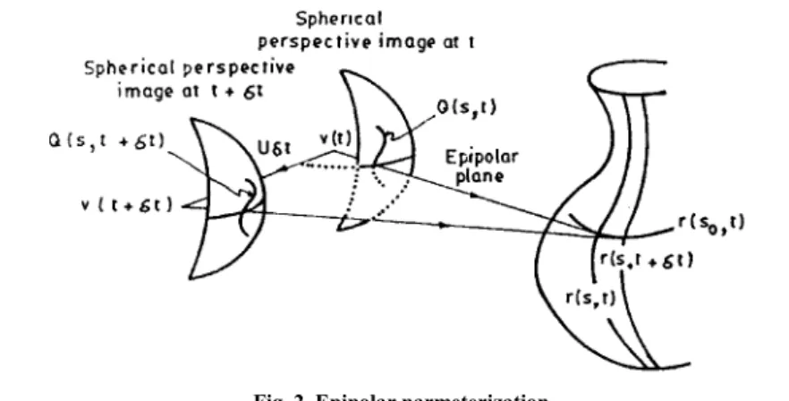
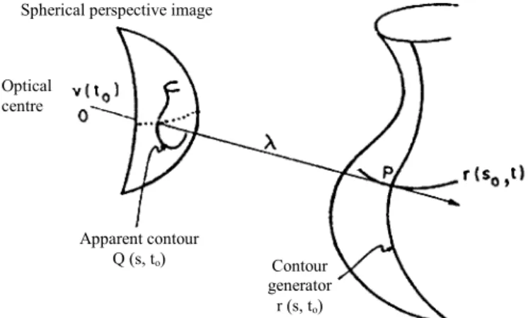
This will make it easier to connect the normal to the surface curve with the normal to the image contour of the same. Note that Q is the direction of the light ray in the fixed reference frame (world frame) R3. It is determined by the spherical image position vector Qc (the direction of the light beam in the camera/viewer coordinate system) and the orientation of the camera coordinate system with respect to the reference frame.
The orientation of the surface normal n can be calculated by measuring the direction of the ray Q from a point on an extremal contour and the tangent to the apparent image contour Qs. The curvature of the apparent contour Kp can be written in terms of its normal and the derivatives of the image curve axis. It can be seen from (1.13) that the frame rate consists of two components: one is determined by the rotational speed of the viewer around the center of the camera and is independent of the structure of the scene (λ).
This relation will give us some quantities with which the coefficients of the quadratic equation describing the surface can be obtained. This result gives a relationship between the derivative of the surface normal and that of the image normal. The normal unit image n can be calculated by measuring the ray direction Q of a point on an extremal contour and the tangent to the apparent image contour Qs.
The sign of the normal can only be determined if we know on which side of the apparent contour the surface lies. However, the "sidedness" of the contour can be determined from the deformation of the apparent contour during the movement of the viewer. Our intention now is to find the variation of n1 along the apparent contour and relate this to the variation in N1 of the contour generator.
Computation of coefficients of quadratic equation
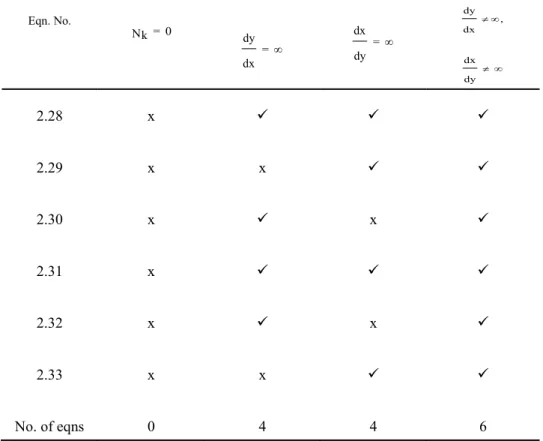
According to the table, at first sight at least four equations can be formed. Let us consider the worst case where the number of unknown coefficients is nine and the number of equations is four. We can form four additional equations by considering the derivatives at a different point in the same view.
But the resulting equations are not independent of the previous equations, hence the need for a second view arises, which can be at any offset and angle from the first view. It can be noted that the first view on the front or top contributes a maximum of 6 equations or a minimum of 4 equations. When two views are taken on the same page, these together would give another equation for depth.
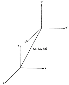
Based on this count, we can get a maximum of 13 equations or a minimum of 9 equations if we take two views on the front and one on the top. Therefore, from 4 views with two on each side, we will get a maximum of 14 equations or a minimum of 10 equations, which includes two equations for different depths. The second view is obtained after rotating the camera in the first view so that the Z-axis points upwards and translation of the origin of the first view point by (' x, ' y, ' z) as shown in Fig.
Computation of depth at a point
Curvature characteristics
The curvature of the apparent contour K along the s parameter curve in the first view is given by . Similarly, the curvature of the apparent contour along the t-parameter curve in the second view is given by . Note that rs and rss are first and second order derivatives of r along the s parameter curve.
The Gaussian curvature can be expressed as the product of the normal curvature Kt and the apparent contour curvature Kps scaled by the depth λ1. The K1 and K2 values provide qualitative information about the intersection point on the element surface patch [23].
Algorithm
Results of Implementation
Simulated object
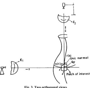
The parameter `s' of the B spline point at the intersection of image curves QF in the front view is obtained as 82,599. The same steps as performed in the front view case are repeated for the image contour in the top view, where QT is the intersection of the image curves. If K1, K2 > 0 the surface point is elliptical, as is the case with the spherical object.
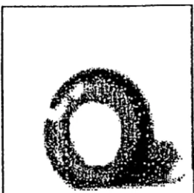
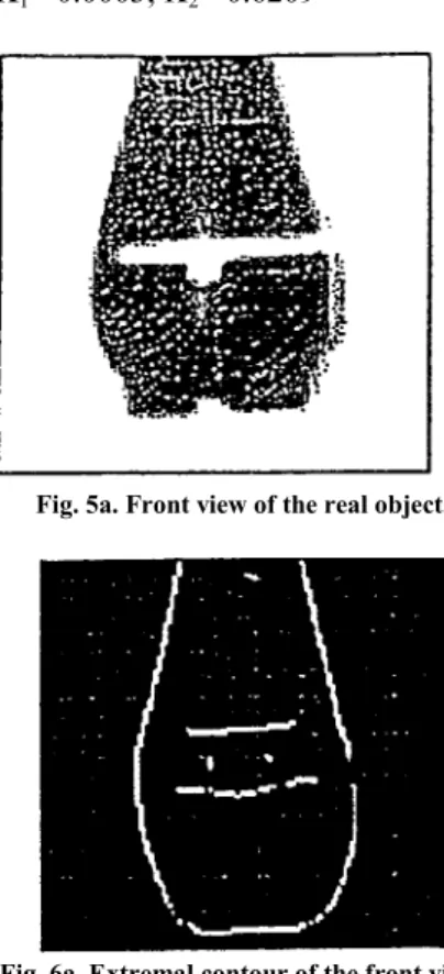
Real object
Since K1#0 this indicates that the nature of the surface is parabolic, as is the case at the point of interest. The coefficients of the quadratic equation provide the structure of the middle part of the object and the other two parts could not be modeled from the second view due to the inaccessibility of corresponding extreme contours. However, these can be obtained from the first view, since the chosen object belongs to the revolution bodies.
Conclusion
Although the proposed method is powerful in terms of surface reconstruction, it cannot provide information on concave surface patches since the curves painted on them cannot be observed as extreme contours. In such cases, information from other curves is extremely important even though this information is not as powerful as that from the extreme contour case. The current method is also not suitable for highly asymmetric surfaces for which a large part of the mesh painted on it would be invisible when the rays from the camera graze it.
The authors would like to express their gratitude to Mr. J.S.Kodamala for the computational assistance provided during the implementation of the proposed methodology.
ةدﺪﻌﺘﻣ ﺪﻫﺎﺸﻣ لﻼﺧ ﻦﻣ ﺔﻧﻮﻠﻤﻟا تﺎﻴﻨﺤﻨﻤﻟا ﺔﺣﺎﺴﻣ ءﺎﻨﺑ ةدﺎﻋإ
ﻮﻟﺪﻧﺎﻤﻧﺎﻫ ﻮﺳاﺪﻣ ،
مار ﺎﺘﻧﺎﺷ .ف و
ﺎﻨﺷﺮﻛ ﻲﺴﻣﺎﻓ .م
ﺎﻳﺪﻴﻣ ﱵﻠﻣ نﻻﺎﺟ ، ﺎﻳﺪﻴﻣ ﱵﻠﻣ٦٣١٠٠
ﺎﻳﺰﻴﻟﺎﻣ ،ﺮﳒﻼﻴﺳ ،ﺎﻳﺎﺟ ﱪﻳﺎﺳ
تارﺎﻘﻟا ﱪﻋ ﺔﻴﻜﻳﺮﻣﻷا ﺔﻌﻣﺎﳉا ،تﺎﻣﻮﻠﻌﳌا ﺎﻴﺟﻮﻟﻮﻨﻜﺗ ﻢﺴﻗ *١٢٦٥٥
نﻮﺳﺮﻔﻴﺟ عرﺎﺷ بﺮﻏ
ﺔﻴﻜﻳﺮﻣﻷا ةﺪﺤﺘﳌا تﺎﻳﻻﻮﻟا ، سﻮﻠﳒا سﻮﻟ
٥٢٣٠٠١ﺪﻨﳍا ،ﺶﻳداﺮﺑارﺪﻧا ،
ﺚﺤﺒﻟا ﺺﺨﻠﻣﻞﺛﺎﳑ دﺎﻌﺑﻷا ﻲﺛﻼﺛ ﻢﺴﺟ ﻂﻴﳏ ﻰﻠﻋ ﻢﺋﺎﻘﻟا ﻂﳋا
ﻂﻴﶈ بﻮﺴﶈا ﻢﺋﺎﻘﻟا ﻂﺨﻠﻟ
ﻩﺬﻫ ﻞﻤﻌﺘﺴﺗ .ﻲﺟرﺎﳋا ﻂﻴﶈا ﻰﻠﻋ ﺔﻄﻗﺎﺴﻟا ﺔﻌﺷﻷا ءاّﺮﺟ ﻦﻣ ﺔﻳدﺎﺣﻷا ةﺮﻜﻟا ﻰﻠﻋ ﻂﻘﺴﳌا وذ ةرﻮﺼﻟا ﻊﻃﺎﻘﺘﻟا ﺔﻄﻘﻨﻟ ﺪﻫﺎﺸﻣ ﺔﺛﻼﺛ ﱃإ جﺎﺘﳓ .ﺔﻴﻋﺎﺑﺮﻟا تﺎﺣﺎﺴﳌا تاﲑﻐﺘﻣ جاﺮﺨﺘﺳﻻ ﱄﺎﳊا ﻞﻤﻌﻟا ﰲ ﺔﻘﻴﻘﳊا
ةرﻮﺼﻟا تﺎﻄﻴﳏ ﻰﻠﻋ ﻢﺋاﻮﻘﻟا ﻂﺑر ﻦﻜﳝ ،ﻚﻟذ ﺪﻌﺑ .ﺔﻴﺟرﺎﳋا تﺎﻄﻴﶈا بﺮﻘﺑ ةﺮﻫﺎﻇ تﺎﻴﻨﺤﻨﳌا رﻮﺻ ﺔﻄﻘﻨﻟا ﺪﻨﻋ ﺔﺣﺎﺴﻤﻠﻟ ﻲﻋﺎﺑر ﻞﻴﺜﲤ ءﺎﻄﻋﻹ ﻲﲰﺮﻟا ﻞﺿﺎﻔﺘﻟا ﺔﻄﺳاﻮﺑ تﺎﻴﻨﺤﻨﳌا ﺔﺣﺎﺴﻣ ﻰﻠﻋ ﻢﺋاﻮﻘﻟﺎﺑ