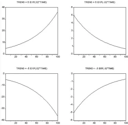
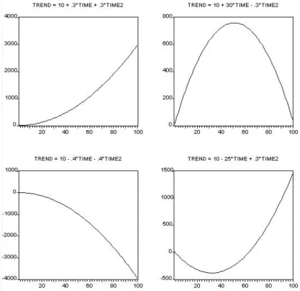
A variety of different nonlinear quadratic trend shapes are possible, depending on the signs and magnitudes of the coefficients. To operationalize this, we use the density prediction N(ˆyT+h,T,σˆ2), where ˆσ2 is the square of the standard error of the regression. Armed with the density forecast, we can set up any desired interval forecast. interval prediction ignoring parameter estimation uncertainty is yT+h,T ±1.96σ, where σ is the standard deviation of the disturbance in the trend regression.
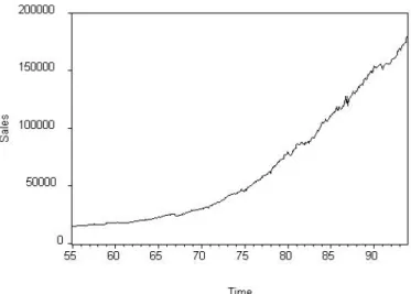
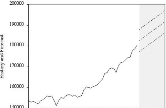
To make this operational, we use ˆyT+h,T ±1.96ˆσ, where ˆσ is the standard error of the regression. We will illustrate trend modeling with an application for forecasting the US. In Figure 5.3 we provide a time series plot of retail sales data, which shows a clear non-linear trend and not much else. The trend appears highly significant as judged by the p-value of the t-statistic on time trend, and the R2 of the regression is high.
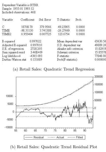
First, we will do so by OLS regression of the log of retail sales on a constant and linear time trend variable. But it is difficult to compare the log-linear trend model with the linear and quadratic models because they are in levels, not logs, making diagnostic statistics such as R2 and the standard error of the regression incomparable. So far, we have been informal in our comparison of the linear, quadratic, and exponential retail sales trend models.
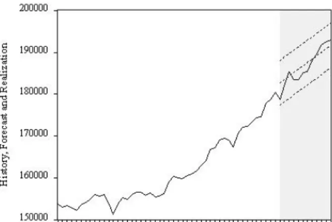
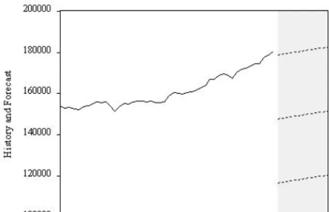
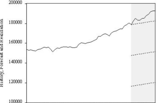
The large predicted decline relative to the pattern's past path occurs because the linear trend at the end of the pattern is far below the pattern's path. The confidence intervals are very wide and reflect the large standard error of the linear trend regression relative to the quadratic trend regression. The reason linear trend forecasting fails is that the forecasts (point and interval) are calculated assuming that the linear trend model is actually the true DGP, when in fact the linear trend model is a very poor approximation of the trend. in retail.
Deterministic Seasonality
For example, people want to take more vacation trips in the summer, which tends to increase both the price and quantity of gasoline sales in the summer. D1 indicates whether we are in the first quarter (it is 1 in the first quarter and zero otherwise), D2 indicates whether we are in the second quarter (it is 1 in the second quarter and zero otherwise) and so on. These different intercepts, the γi's, are called the seasonal factors; they summarize the seasonal pattern over the year.
In the absence of seasonality, the γi's are all the same, so we drop all seasonality dummies and instead include an intercept in the usual way. Before we can estimate seasonal models, we need to create and store seasonal dummies Di, i = 1, .., s on the computer. We will use the seasonal modeling techniques that we have developed in this chapter to build a forecast model for housing starts.
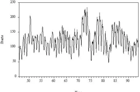
Housing starts are seasonal because it is usually preferable to start houses in the spring so that they are completed before winter arrives. We have monthly data on the US. The numbers show that there is no trend, so we will work with the purely seasonal model. The twelve seasonal dummies account for more than a third of the variation in housing starts, as R2 = .38.
At least some of the remaining variation is cyclical, which the model is not designed to capture. The adjusted values go through the same seasonal pattern every year - there is nothing in the model other than deterministic seasonal dummies - but the rigid seasonal pattern captures a large part of the variation in housing starts. However, it does not capture all of the variation, as is evident from the serial correlation evident in the residuals.
The estimated seasonal factors are just the twelve estimated coefficients on the seasonal dummies; we draw them in Figure 5.16. The seasonal effects are very low in January and February, then increase rapidly, reaching their peak in May, after which they decrease, first slowly and then abruptly in November and December. In Figure 5.17 we see that the housing history starts through 1993, along with the out-of-sample point and the 95% interval extrapolation forecasts for the first eleven months of 1994.
The forecasts look reasonable, as the model has apparently done a good job of capturing the seasonal pattern. However, the prediction intervals are quite wide, reflecting the fact that the seasonal effects captured by the prediction model only account for about a third of the variation in the variable being predicted.
Exercises, Problems and Complements
Use the desired model to predict each of the twelve months of the next year. Plot the trend for different parameter values to reveal some of the different possible trend shapes. One way to deal with seasonality in a series is to simply remove and then model and forecast the deseasonalized series.14.
This strategy is perhaps appropriate in certain situations, such as when interest is explicitly focused on forecasting non-seasonal fluctuations, as is often the case in macroeconomics. Seasonal adjustment is often inappropriate in business forecasting situations, however, precisely because interest is usually focused on forecasting all the variation in a series, not just the non-seasonal part. 14 Removing seasonality is called seasonal adjustment. from the change in a series of interest, the last thing a forecaster wants to do is throw it away and pretend it's not there.
Tip: The seasonally adjusted series is closely related to the residual of the regression of the seasonal dummy variable. Search the Internet (or library) for information about the U.S. Census Bureau's latest seasonal adjustment procedure and report what you learn.
Notes