Where the work of others has been used it has been duly acknowledged in the text. This theory remained popular until the late 1920s, when advances in telescope design and the discovery of the period-luminosity relationship provided incontrovertible evidence that the universe was expanding.
A Timeline of the Universe According to the Expanding Hot Big Bang Cosmology
They estimated the background thermal radiation, a relic of the great temperatures in the early universe, to be 5 K (Alpher and Herman, 1948). The decoupling of photons and matter led to the dark ages, when the universe became transparent.
A Brief Summary of Modern Cosmology
A universe with an energy density greater than the critical energy density would eventually collapse in on itself, while a lower energy density would cause permanent expansion. While a flat universe requires a total energy density very close to the critical energy density, baryonic matter is found to contribute only about 5% to the total energy budget.
A BRIEF SUMMARY OF MODERN COSMOLOGY 7 the required energy in the universe. It must be noted that when Einstein originally used the pa-
These problems, among others, suggest that the standard hot Big Bang (ΛCDM) cosmology may still require some modification. There are now several variations of this theory, but the fundamental proposition is that the universe went through a period of rapid, exponential expansion in the first moments after the Big Bang.
A BRIEF SUMMARY OF MODERN COSMOLOGY 9
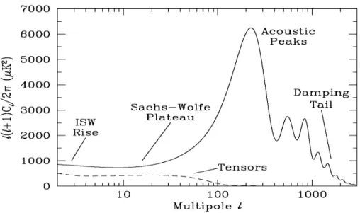
The Cosmic Microwave Background
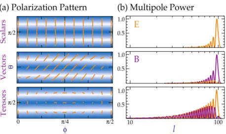
The first experiments to resolve the first peak of the CMB temperature power spectrum were the balloon-borne experiments BOOMERANG (de Bernardis et al., 2000) and. This is because CMB polarization is a direct result of the CMB photons scattered during recombination and escape from the primordial fluid, providing an image of the surface of the last scattering.
A BRIEF SUMMARY OF MODERN COSMOLOGY 13 ing the electron from an overdense region, indicated by thin red lines, will cause the electron to
A Brief Summary of Contemporary Experiments
The depolarizing effect of Faraday rotation can be estimated, given sufficient data at different frequencies (Taylor et al., 2009). A major survey of the area between C-BASS and WMAP is the CMB Q-U-I JOint TEnerife (QUIJOTE) experiment (G'enova-Santos et al., 2015a), which at 10-40 GHz, will provide constraints on the plane component first AME.
GALACTIC FOREGROUND EMISSION 17
Galactic Foreground Emission
Free-Free Emission
The random nature in which the ionized particle interactions occur means that free–free radiation is unpolarized, and it has a spectral index in the optically thin regime of β = −2.1 at GHz frequencies that steepens slightly. The free-free emission spectrum is very well defined by a simple power law, T =νβ, making it one of the most stable solutions for component separation analysis (Planck Collaboration et al., 2014a).
Synchrotron Emission
Synchrotron radiation is strongly polarized with an intrinsic polarization of 70–75%, oriented perpendicular to the projected magnetic field in the source region, and observed polarizations in excess of 30%. Faraday rotation is a frequency-dependent rotation of the polarization angle of an electromagnetic wave propagating through a magnetic field.
Thermal Dust Emission
This is a major source of uncertainty when modeling foreground components, and C-BASS maps will add essential information in the quest to constrain the spectral index of synchrotron radiation across the sky. The intrinsic polarization is reduced by the superposition of different magnetic field lines along the location line, as well as by Faraday rotation.
GALACTIC FOREGROUND EMISSION 21 temperature of 19.6 K. They also found that the mean SED increases with decreased frequency
Anomalous Microwave Emission
Draine and Lazarian (1998a,b) suggested a 'spinning dust' model, in which an electric dipole above spinning dust particles would emit radiation at a frequency related to the spin rate. Later, Draine and Lazarian (1999) suggested another mechanism in which thermal vibrations in ferromagnetic dust particles induce a magnetic dipole emission.
Point Sources and Confusion Noise
The spectral index of the emission measured by the Ring5m experiment was flatter than expected and Leitch et al. 1997) believed that this flatter index was caused by the inclusion of an anomalous component, which is hot (~106 K) free-free emission and flat spectrum synchrotron as possible causes. 2003) also suggested that a flat-spectrum synchrotron would be the likely cause, but the peak spectrum and close correlation with far-infrared templates make this unlikely.
THESIS OVERVIEW 23
Galactic Foreground Removal Techniques
Thesis Overview
In this chapter I describe the objectives and research requirements of the project before providing a detailed description of the experiment itself. In chapter five I describe the commissioning of the southern instrument, as well as the RFI environment in Klerefontein.
The C-Band All Sky Survey
During my PhD, I participated in ordering the southern system and data analysis with both the northern and southern systems. The Northern receiver was completely analog and was forced to use notch filters to remove RFI dominated frequencies.
THE C-BAND ALL SKY SURVEY 27
Science Goals
This requires a more precise measurement of the foreground signal than is currently available (Kogut et al. By accurately measuring the Galactic synchrotron signal at 5 GHz, C-BASS will provide a vital link between other experiments in the seen at low frequency such as the 408 MHz Haslam Experiment (Haslam et al. 1981)) and the 1.4 GHz Dominion Radio Astrophysical Observatory (DRAO) observation (Wolleben et al. 2006)) and limited in-plane microwave frequency experiments dust seen as Wilkinson Microwave Anisotropy Probe (WMAHP) maps (Page et al.
Survey Requirements
The primary foreground contaminants are dust and synchrotron radiation, and while synchrotron radiation is dominant at frequencies below that of the CMB, its influence at higher frequencies cannot be ignored. Secondary experiment goals include probing the galactic magnetic field using synchrotron radiation and searching for new regions of anomalous microwave emission.
THE C-BAND ALL SKY SURVEY 29 The central frequency was chosen to be 5 GHz. The total intensity of the Galactic synchrotron
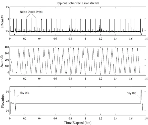
Occasional housekeeping, such as skywatches to monitor gain movements, RFI scans, and directional scans are performed at the observer's discretion. Also note the dips in the sky at the beginning and end of the schedule, with an increase and then decrease in altitude and a corresponding decrease and then increase in intensity while the azimuth remains constant at 0 or 360 degrees.
C-BASS OPTICS 31
C-BASS Optics
Other optical requirements for the secondary mirror included low sidelobe and cross-polarization signal levels and constant phase in the primary mirror aperture. The presence of supports in the dish would have resulted in an increase in cross-polarization and an increase in scan-synchronous ground recording.
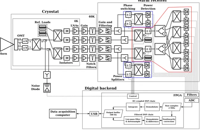
The C-BASS Receiver
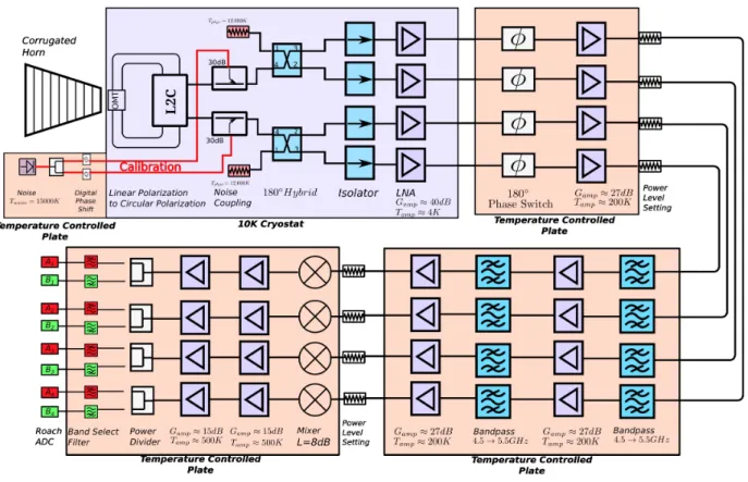
These signals are then amplified and filtered before signal processing and measurement, which is implemented in separate ways by the different receivers. In the northern system, these signals are split into the radiometer and polarimeter branches of the signal chain, as shown in Figure 2.4, taken from King et al.
THE C-BASS RECEIVER 35
Cryogenic Front End
Total Intensity and Polarization Measurement
THE C-BASS RECEIVER 37 while for X and Y linear polarizations
The continuous comparison radiometer differs from the more conventional Dicke switch radiometer (Dicke, 1946), shown in Figure 2.7 (a), because a Dicke switch radiometer switches between air and a reference load, losing half of its observation time. The longer observation time provided by the continuous comparison architecture is especially beneficial for measuring polarization due to the increased sensitivity.
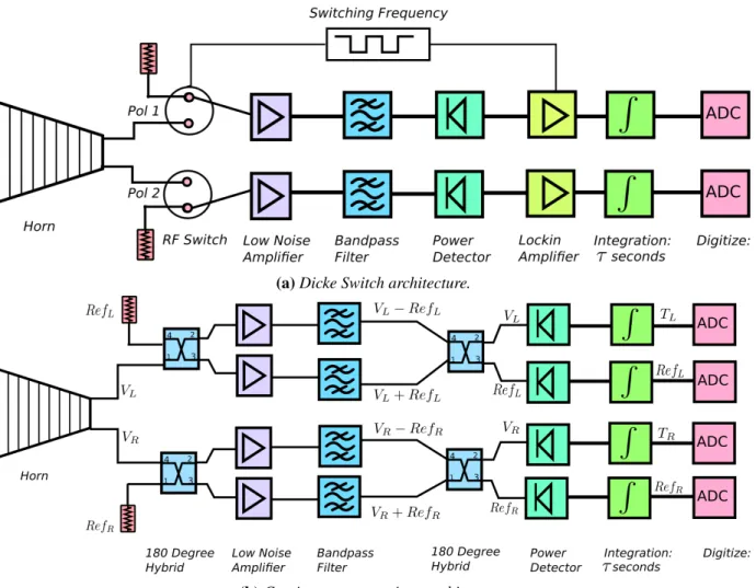
THE C-BASS RECEIVER 39 nals. This measurement is immune to gain drifts in the signal chains as these are uncorrelated
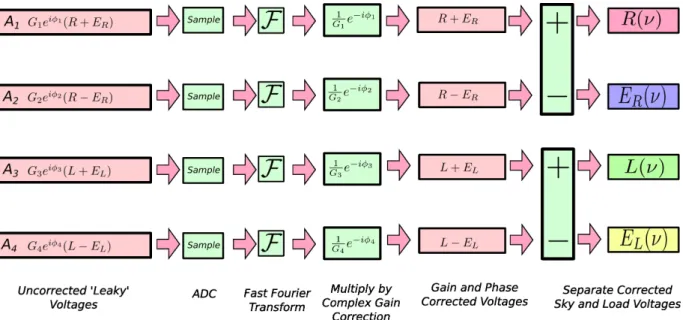
Back End Electronics
This measurement is immune to gain drift in the signal chains as these are uncorrelated. The ROACHs perform the signal processing operations that match the analog radiometer and polarimeter described earlier.
THE C-BASS RECEIVER 41
In this chapter I discuss the analysis of low-level time-stream data from the Northern Telescope. The Southern data analytics pipeline will be similar, but is currently in its infancy and aspects of this will be discussed in the final chapter.
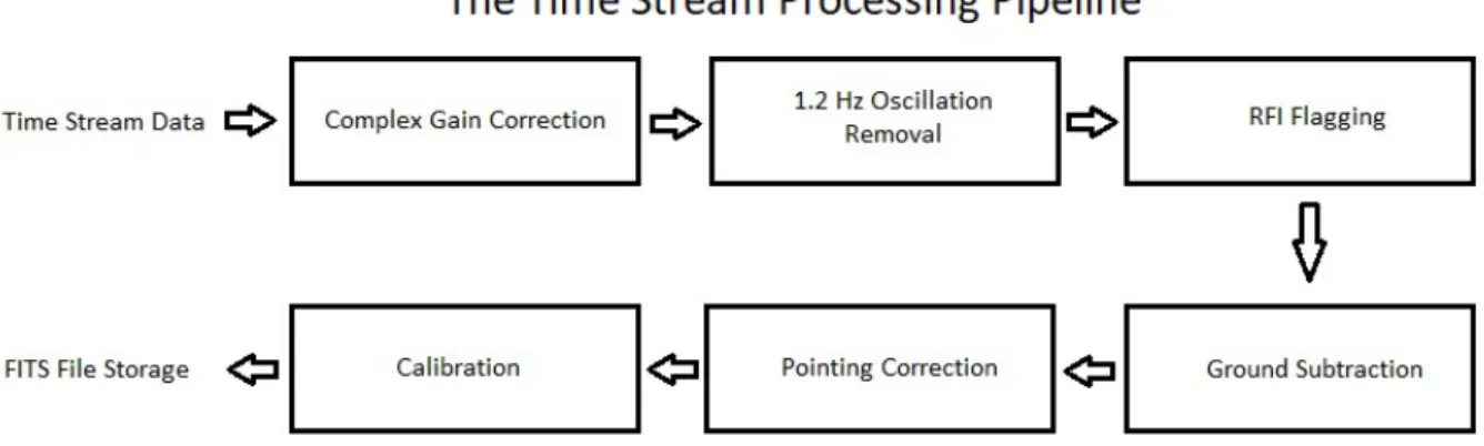
The Time Stream Processing Pipeline
Complex Gain Correction
The complex gain correction stage uses noise diode events to apply a complex gain correction to the data. Thus, any noise diode signal found in the U channels affects the phase of the correction value, which can then be used to correct that leakage.
RFI Flagging
The cryogenic pump that cools the northern cryostat operates with a 1.2 Hz periodic cycle, with the unfortunate side effect of producing microphonic oscillations at 1.2 Hz and its harmonics. A template for the 1.2 Hz oscillations over the course of a schedule is made by analyzing the temperature fluctuations of the cold load.
THE TIME STREAM PROCESSING PIPELINE 45 a particular sample of time ordered data (TOD) to the expected sky signal from our full data set,
This plot illustrates the discretization resulting from using the nearest pixel method with a low-resolution map. TIME-STREAM PROCESSING PIPELINE 47 expected TOD sky signal that actually corresponds to that produced by using the closest.
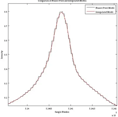
THE TIME STREAM PROCESSING PIPELINE 47 expected TOD sky signal that is effectively the equivalent of that produced by using the nearest
BothM andGare projected in the time domain using map templates and the C-BASS scanning strategy. THE TIMESTREAM PROCESSING PIPELINE 49The cutoff value η started at 6 and was iteratively decreased by 0.5 as in the following process.

THE TIME STREAM PROCESSING PIPELINE 49 The cut-off value η began at 6 and was decreased iteratively by 0.5 as the following process was
For a complete description and example of C-BASS North survey plans, please refer to Figure 2.2 and the preceding paragraph in Section 2.1.2 in Chapter 2. During the marking process, this plan is divided into single azimuth scans and the model is fitted according to equation 3.1.
THE TIME STREAM PROCESSING PIPELINE 51
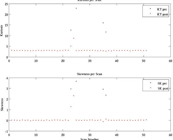
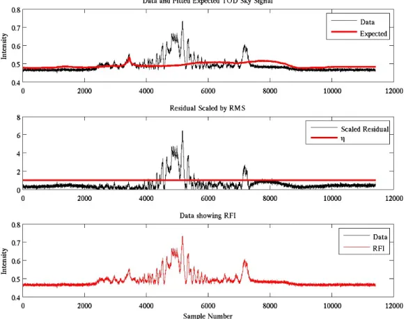
The top panel shows kurtosis before flagging in black, and after flagging in red. The top panel shows the expected TOD sky signal in red fitted to the ordered time data in black.
THE TIME STREAM PROCESSING PIPELINE 53 of data on either side of the RFI events. The bottom panel shows the time ordered data in black
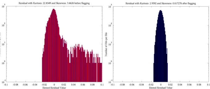
The bottom panel shows the time-ordered data in black. a) Histogram of the residue before marking. b) Histogram of the residue after marking. A collaboration member is currently investigating these small pointing errors, and this part of the marking process will be refined in future versions of the marking routine.
THE TIME STREAM PROCESSING PIPELINE 55
The top panel shows the ordered time data in black and the expected TOD sky signal in red. The middle panel shows the result from equation 3.2 in black and the dashed line η in red.
THE TIME STREAM PROCESSING PIPELINE 57 in detail in Chapter 4
The new routine took just under 12 seconds to score the RFI on this schedule, the old routine took over 380 seconds and ended up scoring almost the entire signal because soil contamination was not accounted for correctly. In fairness, the old method was incomplete and the co-op member who had worked on it left the co-op shortly after I started working on C-BASS.
THE TIME STREAM PROCESSING PIPELINE 59
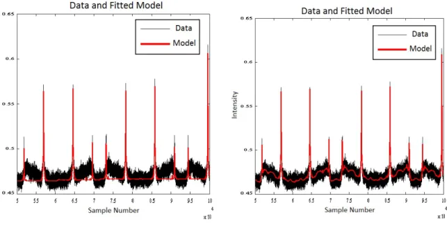
Note that the basis term in the labeling routine had to be removed, resulting in a worse fit between the expected signal and the data. TIME STREAM PROCESSING PIPELINE 613.1.3.1 Effect of Ground Signal on RFI Marking Routine.
THE TIME STREAM PROCESSING PIPELINE 61 3.1 The Effect of the Ground Signal on the RFI Flagging Routine
The panel on the left shows the expected TOD air signal fitted to the time ordering data without including soil contamination. The panel on the right shows the expected TOD air signal fitted to the time-ordered data with the ground pollution signal included.
THE TIME STREAM PROCESSING PIPELINE 63
Pointing
Calibration
Time Stream Processing Pipeline Output
PRODUCING A FINAL DATA SET 65
Producing a Final Data Set
FUTURE WORK 67
Future Work
Two map making programs are currently being tested and will be described in the next section. I will also discuss some of the data consistency tests that were performed to ensure the scientific quality of our data.
Map Making
The angular power spectrum of the map produced using this method is determined using pseudo-C` Monte Carlo methods (Szapudi et al. MAP MAKING 71 the need for multiple iterations, may result in distortion of the TOD signal as a time course.
MAP MAKING 71 the need for multiple iterations, it can result in the distortion of the TOD signal as time stream
Map Making with Ninkasi
When the noise is negatively correlated with the signal, the variance of the measurement will be low, resulting in that period of data erroneously receiving a higher weight. We reduce the bias effect by subtracting an estimate of the signal from the data before estimating the noise.
Map Making with DESCART
This is induced in the map by noise fluctuations in the time stream data as the noise is sometimes positively correlated with the signal, and sometimes negatively correlated. Likewise, a period of data where the noise fluctuation is positively correlated with the signal will erroneously receive a low weight.
MAP MAKING 73
Convergence Tests
The first series started with an input map made from six months of data, denoted here as (O). This output is the difference between the input map (or best guess model) and the data.
MAP MAKING 75 smoothing the mask by the C-BASS beam, calculating the power spectrum of the masked map
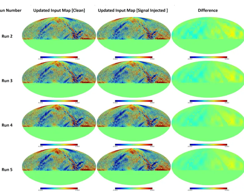
In the case of a successfully converged map, the sum of the Ninkasi output maps R1+..+Rn from the second series of runs would compensate (and therefore remove) the injected artificial signalS. The input maps used in several implementations for the clean and signal-added Ninkasi arrays are shown in Figure 4.3, with the clean maps in the left column, the signal-added maps in the center column, and the difference.
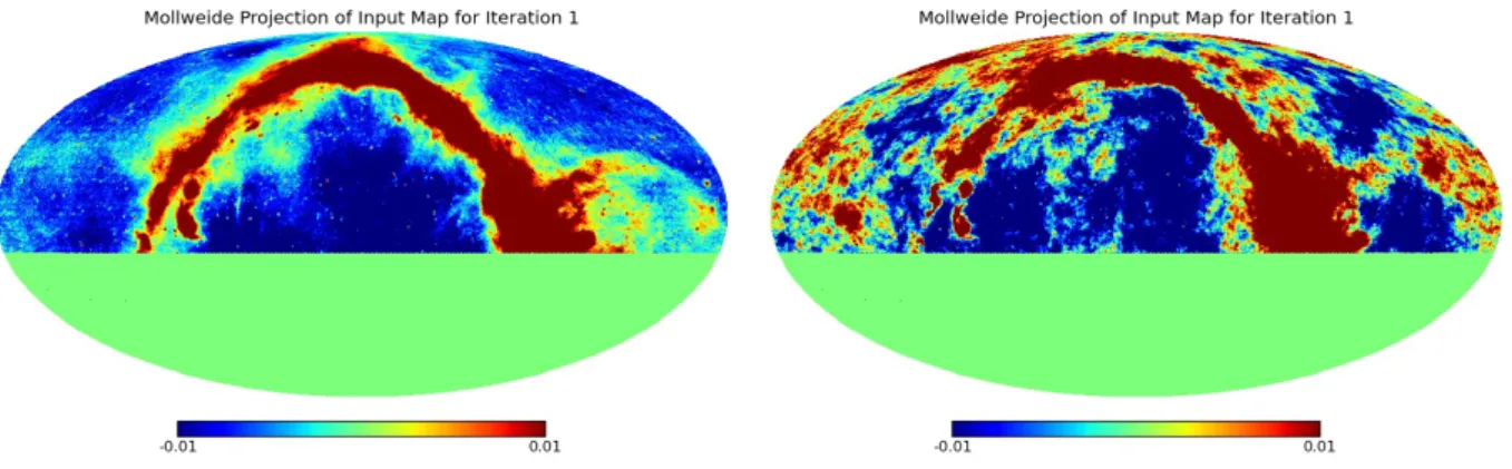
MAP MAKING 77 between them in the right column. This whole process was repeated for Stokes I, Q and U
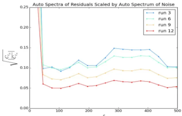
If the residual's autospectrum was of similar order to that of the artificial signal, then the injected artificial signal (or at least a large part of it) persisted and the maps were not converged. This was further tested by taking the cross-correlation of the residual signal and the injected artificial signal.
MAP MAKING 81 The polarization maps were tested in the same manner, where input maps of Stokes Q and
MAKING MAPS 81 The polarization maps were tested in the same way, where the input maps of Stokes Q and. a) Clear the input map (O) before the first start. MAKING MAPS 83Figures 4.9 and 4.10 show the input maps used for each successive run, as well as the differ-.
MAP MAKING 83 Figures 4.9 and 4.10 show the input maps used for each successive run, as well as the differ-
This trend is confirmed when looking at the power spectrum of the residual as shown in Figure 4.11, which shows the auto spectra of the residual as well as that of the injected artificial signal. The requirement that the residuals be small relative to the artificial signal is confirmed in Figure 4.12 where the power spectrum of the residuals is scaled by the power spectrum of the injected artificial signal.
MAP MAKING 85
Data Consistency Tests
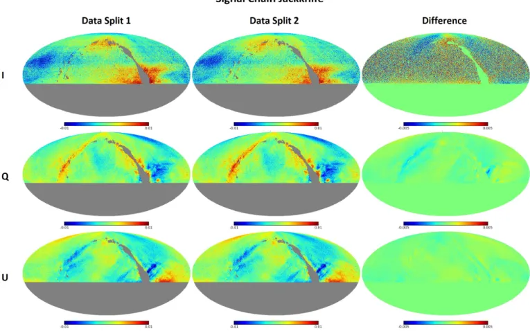
Jackknife Results
We then calculated the power spectra of the two original data splits as well as the power spectrum of the remaining signal after separating the split datasets. Finally, we compared these power spectra and looked for cases where the power spectra of the two data splits varied greatly, resulting in spikes and other features.
DATA CONSISTENCY TESTS 89
DATA CONSISTENCY TESTS 91 schedule, and therefore the higher the RFI flagging fraction, the more unreliable that data would
DATA CONSISTENCY TESTS 93
DATA CONSISTENCY TESTS 95
Note that the power in the Jackknifed dataset was very small, as the power spectra of the two subsets of the dataset were almost identical. This is particularly evident for Stokes' Q and U, where the power spectrum of the Jackknifed dataset is much lower than both subsets.
DATA CONSISTENCY TESTS 97
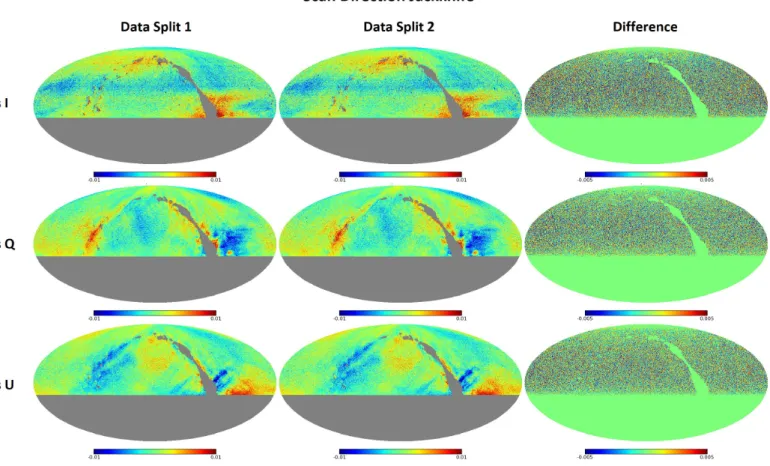
The scan direction jackknife test would fail if there were directional inaccuracies in the data, and given the fact that directional inaccuracies are encountered during the RFI reporting process, as discussed in Chapter 3, it may seem strange that there is no evidence of them in these results. This will be worth investigating further once the pointer inaccuracy is addressed in the low-level timeline processing pipeline.
SUMMARY AND CONCLUSIONS 99
Summary and Conclusions
Knife tests have shown that some considerations must be made when choosing which data to include in the map, as some schedules that contain a large amount of RFI are unreliable and contain bad data. Knife tests showed that the low-level data analysis pipeline improved the quality of our data.
Commissioning the Southern System
Once the receiver had arrived in Klerefontein, it had to be tested to ensure it had survived the journey without damage. We placed the receiver on some scaffolding, far enough from the antenna that it is not affected by its presence.
COMMISSIONING THE SOUTHERN SYSTEM 103 tests were also conducted by covering the receiver with a thick sheet of eccosorb to test receiver
Commissioning C-BASS South Optics
The panels of the southern primary reflector had to be adjusted so that the surface conformed to a. USING THE SOUTHERN SYSTEM 105form described by this equation, to focus the reflector.
COMMISSIONING THE SOUTHERN SYSTEM 105 shape described by this equation, in order to focus the reflector
This photo shows the very bottom of the foam cone that holds the secondary reflector in place, the feed horn and the cryostat. One half of the protective casing and part of the primary reflector are also visible.

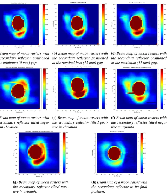
COMMISSIONING THE SOUTHERN SYSTEM 107 gaps of 0 mm, the maximum travel on the bolts (17 mm), and at the nominal focus of 12 mm
COMMISSIONING THE SOUTHERN SYSTEM 107gap of 0 mm, the maximum travel of the bolts (17 mm), and at the nominal focus of 12 mm. a) Beam map of the lunar grid with the secondary reflector placed at the smallest (0 mm) gap. b) Beam map of the lunar grid with the secondary reflector positioned at the nominal best (12mm) spacing. c) Beam map of the lunar grid with the secondary reflector placed at the maximum (17 mm) gap. d) Ray map of the lunar grid with the secondary reflector tilted negatively in height. e) Beam map of lunar rasters with the secondary reflector tilted positively in height. f) Beam map of lunar rasters with the secondary reflector tilted negative in azimuth. g) Beam map of lunar rasters with the secondary reflector tilted positive in azimuth. h) Beam map of a lunar grid with the secondary reflector in its final position.
COMMISSIONING THE SOUTHERN SYSTEM 109
Optical Pointing
COMMISSIONING THE SOUTHERN SYSTEM 111
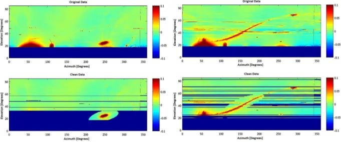
The automated process identified when the telescope was aiming accurately by estimating the maximum brightness near the center of the image and comparing it to the maximum brightness of the entire image. COMMISSIONING THE SOUTHERN SYSTEM 113 near the center of the image, and the data from this list was then analyzed to produce an indicator.
COMMISSIONING THE SOUTHERN SYSTEM 113 near the centre of the image, and the data from this list was then analysed to produce a pointing
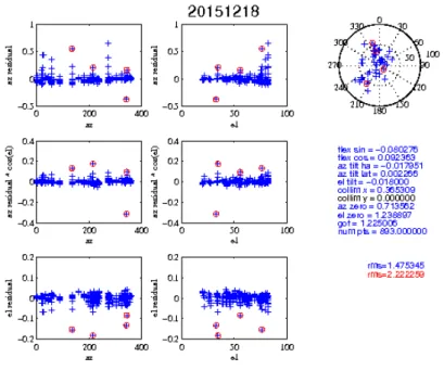
Of particular importance in this figure is the circle in the upper right and the calculated RMS of the heading error (denoted 'space angle' on the graph), in minutes of arc. It also shows the sky coverage, the values of the fitting parameters and the rms of the heading error (denoted 'space angle') in minutes of arc.
COMMISSIONING THE SOUTHERN SYSTEM 115
Radio Pointing
The RFI Environment at Klerefontein
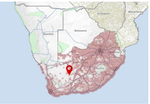
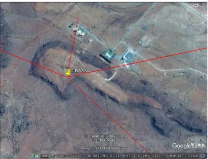
Southern System Commissioning 1175.15 is a Google Earth satellite image of the C-BASS site with ground azimuth directions.
The large vertical streak near azimuth 90 is the firing of the noise diode and can be ignored in this analysis. USING THE SOUTHERN SYSTEM 119 The tremendous advantage of the southern system's digital back end is that the spectral in-.
COMMISSIONING THE SOUTHERN SYSTEM 119 The tremendous advantage of the southern system’s digital back end, is that the spectral in-
Investigating RFI Using the C-BASS Signal Band
COMMISSIONING THE SOUTHERN SYSTEM 121
Summary and Conclusions
SUMMARY AND CONCLUSIONS 123 southern survey will also enable us to deliver full sky maps of Galactic foreground radiation at
First measurements of the polarization of the cosmic background radiation on small angular scales with CAPMAP. Analysis of the accuracy of a destriping method for future cosmic microwave background maps with the PLANCK SURVEYOR satellite.