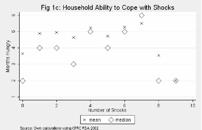
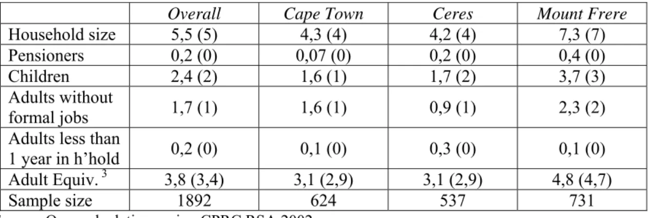
We also observe that the number of adults who joined the household in the past year is insignificant for the median household. In most cases, new arrivals to the household constituted a minority of household members. The survey also collects information on the types of negative shocks that households have experienced in the past year.
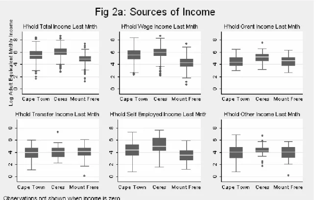
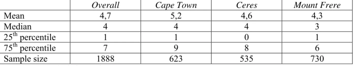
In Cape Town, the average household experienced two types of shocks last year. In Mount Frere, the average household experienced three types of strokes in the past year, and a quarter of households experienced at least four strokes. Our data collect information on income in the past month, as well as income each month during the past year.8 In addition, the survey identifies the source of income for each household in the past month.
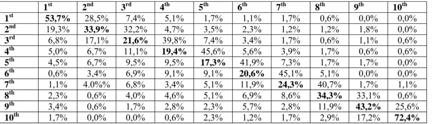
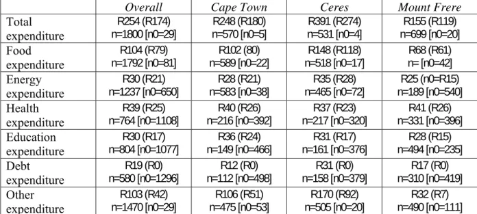
Instead, we show the number of households with zero income separately in the table (if n0=x). Households that remain in the same decile rank when annual income is used instead of last month's income will have a rank change of zero. Households that remain in the same decile are shown (in bold) along the diagonal of the matrix.
This is especially true for households at the top of the distribution where a rank change of more than one decile is unlikely.
3 Expenditure-based rankings
In Ceres, households are more likely to move up, but the result is not as strong as in Cape Town. Interestingly, households in low income deciles and households in high income deciles are more likely to remain in the same rank than households in the middle deciles. Households that move hardly move more than one decile in the distribution (1% corresponds to approximately two households in the decile).
The CPRC survey collects information on 20 expenditure categories per household in the last month. 12 Only 16% of the households in the sample had some savings at the time of the survey. Households in Ceres tend to enjoy higher spending per adult equivalent than in the other two regions.
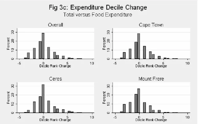
The differences are less stark when food expenditure is used, with poorer households clearly spending a higher percentage of their expenditure on food (and possibly using debt to finance food expenditure). This effect is clearly shown in the graphs where the bottom outliers are reduced when food expenditure is graphed. Mount Frere has consistently been shown to fare worse when spending measures are used to rank households.
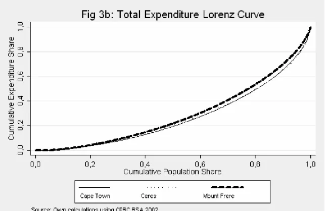
It is not clear whether Cape Town or Ceres is more unequal, as the lines cross in the upper part of the distribution. More surprisingly, households in Cape Town and Ceres are equally likely to fall or improve in the rankings. Here there is a negative bias in the classification of food expenditure as Mount Frere households produce for their own consumption.13.
Households that remain in the same decile are shown (in bold) along the diagonal of the matrix as before. In fact, no household in the bottom decile in terms of total expenditure moves above the 3rd decile in terms of food expenditure. As with income, deciles are least stable in the middle of the distribution, and least stable in the sixth decile.
4 Wealth-based rankings
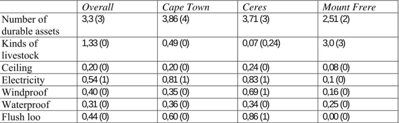
The coefficient (and sign) on the variable is sensitive to which other variables are included in the procedure. Households are then ranked by summing the product of each coefficient on the variable and whether they are above or below the average for that particular variable. The negative sign is simply driven by the fact that households with no livestock (ie not in Mount Frere) tend to be better off.15.
The top left graph shows that less than 30% of households remain in the same decile when classified by household structure alone and not by the composite wealth index. The largest change in the ranking is caused by the classification of households by livestock only, with few households remaining in the same decile. The lower right graph shows the effect of excluding livestock from the composite index on the ranking of households.
The majority of households do not change ranks, but certain households are punished quite severely. However, in Cape Town and Ceres, the majority of households are better off with livestock excluded. This result is consistent with the notion that these households were 'boosted' in the previous analysis.
But a substantial number of households are still growing (i.e. these households had more than the average amount of livestock). 15 Positive coefficients on the livestock variables are only obtained when Mount Frere is run as a separate sample. Negative coefficients are counterintuitive, as the household with more livestock than average will be penalized more than the household with less than average.
This is a consequence of a household without livestock being generally better off than a household with livestock. But it does not follow that families with few livestock are better off than families with many livestock. Conversely, households that have lower than average livestock are unfairly increased in distribution.

5 Comparing the three measures
It is therefore clear that our principal components technique struggles to accommodate a rural-urban divide, as it does not arrive at meaningful coefficients for the livestock variables. This effect is marginal in the higher deciles, but penalizes certain above-average households in the lower deciles. This is the only case where our poverty measure has difficulty identifying the lowest point of the distribution.
There is not much difference whether looking at fixed assets or structural assets. From Figure 5b it appears that households in Mt Frere are more likely to move up in relative ranking when the Alternative Wealth Index is used instead of last month's income, but the effects are not overwhelming and a large number of households in each location move up as well as down. The most penalized area is Cape Town, where significantly more households fall in the rankings when an asset-based measure is used.
The transition matrix of total versus alternative wealth rankings (see Table 5a) shows significant changes in household rankings at the lower end of the distribution.
6 How well do these measures ‘explain’
All assets included in our asset index are illiquid in the sense that they are difficult to convert into cash. An additional question is how households finance their assets and what impact this has on their ability to service basic needs.
7 Poor by All Accounts: Developing Composite Indicators
The composite index is less useful in explaining household hunger, and only in the bottom half of the sample (i.e. households that are in the bottom 40% at least three times) do we see a positive relationship between hunger and the index. This works indirectly with the finding that the money metric measures. and not wealth measures) are important in explaining household hunger, but that wealth-based measures could help explain more long-term dimensions of poverty.
8 Conclusion