In chapter 2 of this thesis, we present a basic overview of the software package Mathematica focusing on its structure and capabilities. In §2.1 we provide a brief background on Steven Wolfram who was instrumental in the creation of this software package. The graphical user interface is explored in §2.3 with some of the computing features explained in §2.4.
In §4.2, analytical properties of this equation are reviewed using the Lie analysis of differential equations. The solution of the Emden-Fowler equation is reduced to a simpler second-order autonomous equation.
Chapter 2
Mathematica
The Developer
Overview of Mathematica
The front end, which provides the user interface, is a separate software component from the kernel that performs the calculations. The front end, also called the notebook interface, is the graphical user interface for the Mathematica kernel and is separate from the kernel. The notebook processes text formatting and sends a calculation to the kernel only when requested.
The application program of this software package is developed from a combination of the Mathematica language itself and the C programming language. To continue working on a previously saved notebook, it must be retrieved and evaluated (i.e. each line of input processed by kernel) to use previous variables or values in the new Mathematica session.
User Interface
Once you're in Mathematica, you can get help on built-in functions, add-ons, getting started/demo, and other information. Additionally, the Mathematica book is available online for explanations, detailed examples, and syntax on built-in functions. At the end of each Mathematica session, the notebook can be saved for future use, and the program can be terminated using the Exit option on the File menu.
There are many different palettes that have buttons that can be selected to produce the syntax of built-in functions and special symbols. When the Mathematica icon is clicked, the user interface portion of the program is loaded.
Computational Features
Most of the arithmetic operators and standard mathematical functions can work with symbolic expressions as well as with numeric expressions. The graphical capabilities of Mathematica are one of the features that have contributed greatly to its success. Furthermore, the axis labeling of the indices for the bitmap format is not clear and as a result all graphs in subsequent sections have been performed using the metafile format.
It is possible to stop Mathematica in the middle of a calculation if it is taking too long to produce a result, using the Interrupt Evaluation. When Mathematica simplifies an expression such as x + x to 2x, it treats the variable x in a purely symbolic way.
Mathematica Resources
Add-on Packages
To load a package, a name and path must be specified using the following syntax. One of the functions inside the DiscreteMath package is called Subfactorial and can be used as follows after loading the package.
A Tour of Mathematica
Mathematica returns approximate numerical results just as a simple calculator would by using the I IN, operator. Extreme care must be taken in using this command as j(1- .r)2 and j(x - 1)2 will always give different results. To access the fifth element of the list, we use two square brackets to enclose the index.
Mathematica has a built-in function called Table that can be used to generate lists In[20]:= Table[n!, {n,1,S}]. Another type of plot that can be used to represent a list of numbers is the ListPlot.
Commands Frequently Used in this Thesis
For example, drawing a three-dimensional graph for the function sin(x + sin(y)) is obtained via NDSolve[eqns, y, {x, xmin, xmax}] finds the numerical solution of the ordinary differential equations eqns for the function $y$ with the independent variable $x$ in the range xmin to xmax. NDSolve[eqns, y, {x, xmin, xmax}, {t, tmin, tmax}] finds the numerical solution of partial differential equations.
Infinity maximum size of each step Automatic accuracy figures sought Automatic initial step size used. NOSol ve follows the general procedure of reducing the step size until solutions are closely monitored. To avoid this problem, the default setting for MaxSteps is 1000 for ordinary differential equations and 200 for partial differential equations.
In some cases, the very first step size that NDSol ve takes can be as well. To avoid this problem, the StartingStepSize option can be set explicitly to specify the size to choose for the first step. The RKSolve function is an implementation of the Runge-Kutta method for finding numerical solutions to ordinary differential equations.
This function was used to verify all the results obtained in Chapter 3 and some results in Chapter 4 via NDSolva. Using the syntax already given for RKSolve, the Mathematica command for (2.5) with the given initial conditions translates to. After introducing the package and explaining the commands used to obtain the results in this thesis, we can present these results.
Chapter 3
Orbit Equations
- Introduction
- Newtonian Equation
- Relativistic Equation
- Numerical Approach
- Perturbative Approach
- Chapter 4
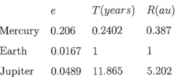
Then the conservation of angular momentum and the conservation of energy generate the equation. where y = 1/r, E is the energy of the circuit, h is the angular momentum per unit mass, G is the universal gravitational constant and the prime denotes differentiation with respect to the x -angular displacement. Despite the nonlinearity of equation (3.1), Mathematica is still able to provide closed-form solutions. To obtain physically meaningful results, we need to solve (3.10) subject to the initial conditions.
Unfortunately, we cannot continue with the equation and initial conditions in this form due to the presence of relatively large numbers. We will always choose the lower value of y(O) to be consistent with our choice of origin. To obtain a more meaningful, visual interpretation of the motions of these planetary bodies, we generate graphical representations of and (3.17).
Consequently, we use PolarPlot to obtain an accurate reflection of the motion of these objects. These treatments provide detailed arguments about the physical meaning of the relativistic equation (3.18) for planetary orbits. We start with (3.13) because of its simplicity and the presence of an analytical solution to verify the numerical results.
To determine the behavior of the graph, we now examine Mercury's orbit by looking at a small portion of the graph. It is clear that while the graphs for the relativistic case appear to be a solid line, the thickening is due to a precession of the planetary orbits. Again due to the presence of relatively large numbers, we rescale (3.23) using the transformation given in (3.12) to produce
Since (3.33) is a linear equation in wl/ we can write . where Wa) Wb and Wc are solutions of the equations. This is surprisingly since E « 1 after considering the physical values of the various constants.
Emden-Fowler Equation
Introduction
Lie Analysis
- et = 0 and ~ = 0
- a = 0 and ~ > 0
- a = 0 and ~ < 0
- a > 0 and ~ = 0
- a > 0 and ~ < 0
- a = 5VK and ~ > 0
- a = -5VK and ~ > 0
- a < 0 and ~ = 0
- a < 0 and ~ < 0
- Discussion
A systematic method for determining whether a second-order differential equation can be solved by quadratures is the Lie method. Lie analysis was first used by Kustaanheimo and Qvist (1948) in this context to analyze propagating inhomogeneous models; they considered the case a = 0 and C = O. They also commented on the general integrability of this equation for other values of a and~.
Given the importance of a and ~ in the behavior of the solution of (4.20), we consider numerical solutions to (4.20) for all possible classes of values of a and. For each of the above cases, Mathematica was used to numerically solve the respective equation using the NDSol ve function. All solutions obtained via the NDSol ve function were verified using the RKSol ve function discussed in Chapter 2.
To determine the behavior of the solution for other positive values of et we consider the case when et = 5 and et = 15. To determine the behavior of the solution for the above cases we present a graphic representation below. From the above numerical results it is clear that the behavior of the solutions of equation (4.20) falls into three distinct classes: a = 0, a < 0 and a > O.
As the coefficient of Y' (X) it plays a decisive role in the behavior of the solution of (4.20). Analyzes using the dynamical systems approach in cosmology generate useful results as shown in the works of Billyard et al (1999a, 1999b, 2000). Note that the range of X is calculated via (4.47) and note that x = r2 where r is the radius.
A Particular Example
- c(t) = exp t
- c(t) = sin t
So far the energy density p and pressure p have been generally taken to be c(t) which is an arbitrary function of integration. It is clear from the eight graphs above that both the energy density jl and the pressure p are singular at some t and at some r. For this situation the graphical representation for r = 1 and r = 10 (dotted line) for the energy density is.
It is clear from the energy density and pressure graphs that the different choices for c(t) produce singularities in most graphs.
Chapter 5
Conclusion
However, this program has some flaws that were discovered during the course of this task in some algorithms. In the case of the Newtonian and first-order relativistic equations in Chapter 3, nonsensical results (which are not reported here) were obtained. When we considered the linear versions of the second-order equation, we had no problems.
The analytical algorithms in function D801 have provided simple solutions to a complex equation in Newtonian theory; however, it could not provide meaningful results for the relativistic equation. The ND801 ve command was used to obtain numerical solutions which were then compared with the analytical results. When plotting the graph of the relativistic equation, we saw a clear thickening of the orbits of the planets Mercury, Earth and Jupiter.
A perturbative approach was also used to analyze the relativistic equation for the planet Mercury, verifying the numerical results. We could not notice this effect using the numerical approach for the same range. The numerical amount of perihelion shift was also obtained for the planets Mercury, Earth and Jupiter.
After performing the Lie analysis, we obtained a simple second-order autonomous equation and found that the behavior of the solutions fell into three different classes; 0 and 0: > O. We then generated graphs of the energy density and pressure for a range of values corresponding to radii and time values for different cases that occurred. However, these treatments show that it is in principle possible to investigate these nonlinear gravitational fields, even though the original equation is nonlinear.
Bibliography
