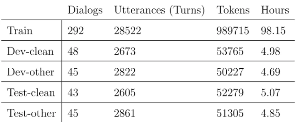
Results are calculated over all development and test distributions of the SAIGEN corpus using oracle SAD. The margin of error is the standard deviation of the mean diarization error between noise levels.
Background
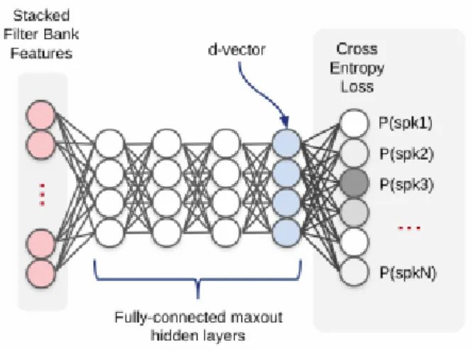
These frame-level speaker embeddings are averaged to form utterance-level speaker embeddings, known as d-vectors, and can be used for speaker diarization and recognition. The ultimate aim of this dissertation is to develop a loudspeaker diarization system which is sufficiently adapted to operate in South African telephone speech, so that the loudspeaker level indexing provided by the system can be used to isolate a specific speaker in a conversation before audio. is transcribed.
Problem statement
Since this small proprietary corpus is not large enough to adequately train a speaker diarization system from scratch, the main research goal is to investigate techniques and methods by which a pre-trained speaker diarization system can be adapted to new, low-resource domains become Additionally, the loudspeaker indices can be used by downstream ASR components for loudspeaker-specific adjustments.
Project scope
Research questions
Objectives
Research methodology
Evaluate the utility of the custom speaker diarization system to improve ASR and speaker indexing. Analysis: Analyze the effects, benefits, and pitfalls of domain adaptation in real-world scenarios, as well as the impact of the adapted systems on downstream applications, such as speaker indexing and ASR.
Dissertation overview
Evaluate and compare state-of-the-art systems and adaptations to the EMRAI synthetic corpus to determine appropriate approaches. Apply these approaches to the SAIGEN corpus to evaluate the efficiency of domain adaptation in a real-world scenario.
Publications
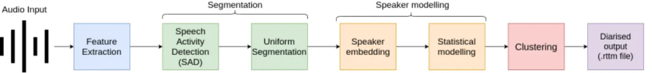
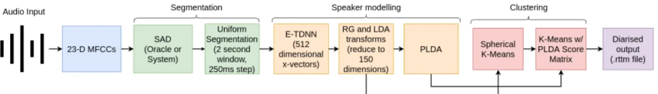
Speaker modeling provides the input to the clustering step (Section 2.6) which uses the speaker embeddings to form groups of speech segments containing the same speakers. Finally, we discuss approaches to domain adaptation (Section 2.5) that are mainly focused on the adaptation of the statistical components.
Feature extraction
Segmentation
Speech activity detection
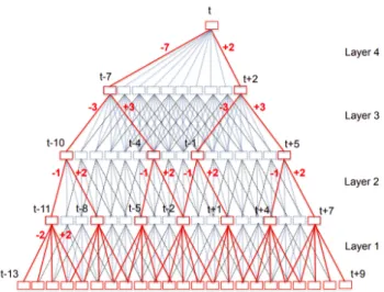
For earlier speaker diarization systems, the modus operandi, in terms of segmentation, was to use Speaker Change Detection (SCD) models. The speaker change points are then placed between all frames that have a speaker change probability higher than a predetermined threshold.
Speaker modelling
Speaker embedding
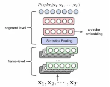
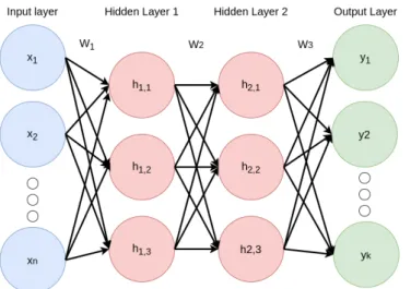
This subsection first describes how an MLP and TDNN work and why the TDNN-based x-vector systems are preferred over the d-vector alternatives. Therefore, we only use x-vector systems in this study, as these are currently the most common.
Statistical modeling
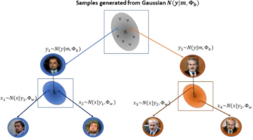
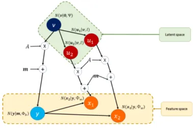
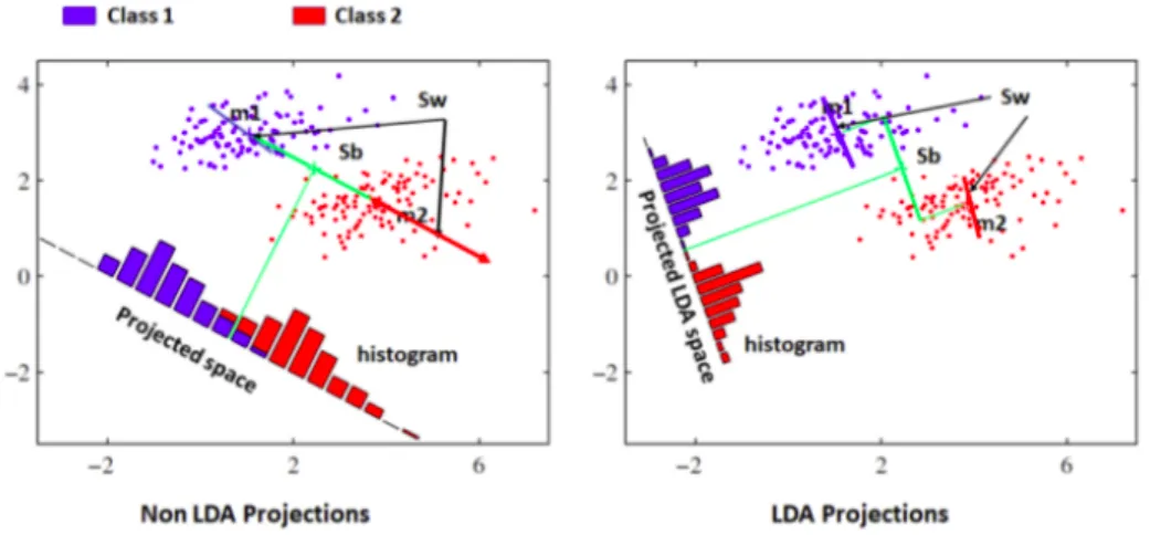
By applying an RG transformation to the x vectors, the covariance matrix of the white x vectors (θ = I) is diagonalized and the dimensions of the x vectors are statistically independent. This is done by defining a latent variable y that represents the mean of a specific class and the center of the mixture component.
Domain adaptation
Adaptation of the RG and LDA transforms
PLDA interpolation
Where ΘW−adapt and ΘB−adapt are the adapted within-class and between-class coordination matrices, ΘW−in and ΘW−out are the ID and OOD within-class covariance matrices, and ΘB−in and ΘB−out are the ID and OOD between- class covariance matrices. The interpolation parameter α ∈ [0,1], is proportional to the contribution of the ID data to the fit and should be fine-tuned on the ID data.
Clustering
K-Means clustering
An important drawback of the K-Means algorithm is that it requires the number of centroids or, equivalently, clusters, to be known. Move each centroid so that it is at the center of all the data points assigned to it.
Agglomerative hierarchical clustering
Variational Bayes Hidden Markov Model clustering
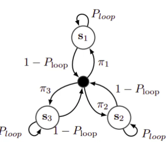
At the same time, the loudspeaker distributions, eg, the distribution of xt, are modeled by a latent vector ys which is of the same six dimensionality. At initialization, the HMM immediately transitions from the non-emitting node to one of the speaker states with probability πs.
Evaluation metrics
Scoring metrics for speech activity detection
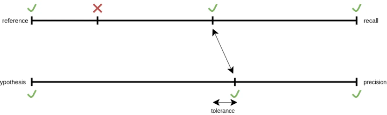
By misclassifying speech segments, the downstream components will not function on all speech segments or they will function on audio segments that are actually non-speech, such as silence or noise. Boundary recall, which compares the amount of hypothesized speech/nonspeech boundaries to the actual speech/nonspeech boundaries.
Scoring metrics for speaker diarisation
DER is most commonly used for evaluating diarization performance and is the primary measure used in the international DIHARD speaker diarization challenges. Missed Detectioni is the total amount of time belonging to speaker i that is not allocated to speaker i.
Toolkits
PyAnnote-metrics
Scikit-learn
Scikit-learn is an open source Python library used for machine learning tasks [61] such as classification, regression and clustering. In this work, we will use Scikit learning to calculate the F1 score for SAD evaluation and for performing AHC and K-Means clustering.
Kaldi
Conclusion
Due to time constraints, the experiments with the EMRAI corpus could not all be replicated on the SAIGEN corpus. Therefore, when the SAIGEN corpus became available, the base systems were chosen based on their performance on the EMRAI corpus.
EMRAI corpus
SAIGEN corpus
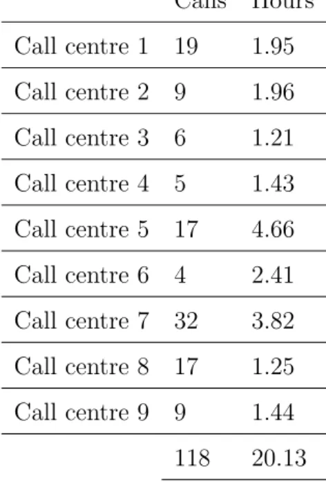
Data collection
Using the diarization output from the baseline system, we identified calls with higher error rates than other calls in the same call center and manually verified the annotations of the identified calls. In most cases, the calls with the highest error rate contained labeling errors or misspellings in the annotations.
Data analysis
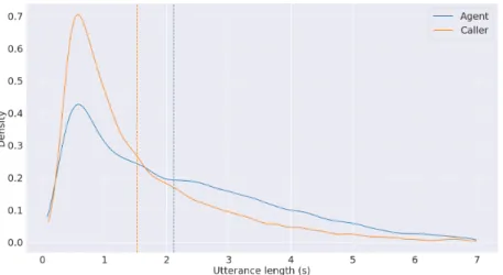
Finally, Table 3.3 shows the composition of speech and non-speech events in the SAIGEN corpus as the average percentage of the total time in which a particular event occurs. Other speech events such as overlapping speech and background speech make up a relatively small portion of the speech.
Introduction
Several pre-trained, state-of-the-art x-vector and SAD models are described, evaluated and compared using the EMRAI corpus. In addition, domain adaptation on the EMRAI corpus is investigated by retraining the RG and LDA transformations and performing PLDA interpolation.
Pre-trained systems
Pre-trained SAD baselines
SAD consists of two bidirectional LSTM layers of size 128 followed by three intermediate layers of the same size [68]. As with TDNN-SAD, this model has two output classes: speech and non-speech.
Pre-trained x-vector models
The E-TDNN network accepts 23-dimensional mean-normalized MFCCs with a frame length of 25 ms extracted every 10 ms. TDNN operates on 40-dimensional, mean-normalized FBanks with a frame length of 25 ms extracted every 10 ms.
![Table 4.1: The network architecture used in the E-TDNN system [69]. K represents the input feature dimensionality, T is the number of input frames and N is the number of speakers](https://thumb-ap.123doks.com/thumbv2/pubpdfnet/10396058.0/71.892.185.709.260.717/table-network-architecture-represents-feature-dimensionality-number-speakers.webp)
Evaluating pre-trained systems
- Experimental setup
- SAD systems: no adaptation
- X-vector systems: no adaptation
- X-vector systems: retrained RG and LDA transforms
- X-vector systems: PLDA interpolation
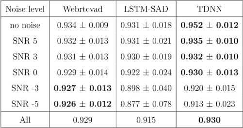
To identify the best performing SAD system, we compare the performance of each pre-trained model on all 6 noise levels of the 'dev-other' subset of the EMRAI corpus. Note that neither pre-trained system clearly outperforms the other two at all noise levels and.
Conclusion
Finally, the use of systems tailored to specific loudspeaker adaptations is investigated using a pre-trained ASR system. Finally, the performance of a pre-trained ASR system is compared with and without the use of system(s) tailored for specific loudspeaker adaptations (Section 5.5).
Experimental setup
After establishing the baseline system, the effects of the default system settings on the diarization error are investigated (Section 5.3). Second, the baseline system is adapted to the SAIGEN domain using retrained RG and LDA transformations and PLDA interpolation and we introduce the use of silhouette coefficients to automatically refine PLDA interpolation on a per-call basis ( Section 5.4).
Baseline diarisation system
- Evaluation of SAD systems
- X-vector segmentation
- SAD segment padding
- Baseline performance
In Chapter 4.3.1, the E-TDNN x-vector system is implemented 'as is', without changing any of the default settings. The TDNN-SAD is chosen for the baseline system because of its performance on the SAIGEN corpus.
Domain adaptation
Retrained transforms and PLDA interpolation
To retrain the RG and LDA transformations, we follow the same process as in Figure 4-1, but we swap the EMRAI corpus for the SAIGEN corpus: we train ID transformations on the development set of the SAIGEN corpus and a OOD PLDA model on the x vectors extracted from the development sets of Voxceleb1 and Voxceleb2 using the ID transformations. For PLDA interpolation, we follow the same process as in Figure 4.2: we train an ID PLDA model on x-vectors extracted from the development sets of the SAIGEN corpus using the ID transformations and interpolate the ID and OOD PLDA models .
Fine-tuning PLDA interpolation using silhouette coefficients
The SC is calculated using the 'score matrix SC' method and the margins of error are the standard error between splits. Similarly, Figure 5.6 shows the probability distribution of the Pearson correlation coefficient between the SC (calculated using the 'score matrix SC' method) and the diarization error for all calls within each split.
Conclusion
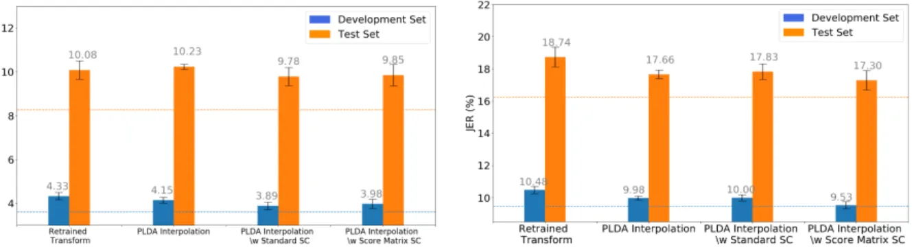
It is also shown that using the PLDA score matrix to calculate the SC performs slightly better, in terms of mean JER, than using the cosine distance between embeddings (Figure 5.3). As shown in Table 5.5, using the SC to refine the PLDA interpolation process, especially the 'Score Matrix SC' method, yields the highest relative increase in diary performance over the unadjusted baseline (in terms of mean JER ).
Key findings
Although the SAIGEN corpus was considered to represent a single domain—South African call centers—the calls within the dataset contained minor domain discrepancies, such as differences in non-speech types, languages, and recording conditions. Further investigation is needed to determine whether using SC to fine-tune the interpolation process is a practical solution in cases where the ID data is slightly inconsistent.
Addressing research questions
Does the SAIGEN corpus contain sufficient data for domain adaptation of a pre-trained system? However, the use of loudspeaker diarization in ASR depends on the basic performance of the ASR system.
Practical Implications
The observed improvements were small compared to the improvements of the speaker dialog system before and after adaptation. The custom speaker diarization systems can also be beneficial for downstream ASR systems that require speaker indices for speaker-specific adaptations, depending on the specific ASR system and other environmental factors such as target data.
Future research
The domain matching methods for speaker diarization systems investigated in this research can be used for improved speaker indexing in unlabeled ID data. It should be investigated whether SC can be used to automatically fine-tune other hyperparameters such as default system settings.
Conclusion
Robust DNN Embeddings for Speaker Recognition", in 2018 IEEE International Conference on Acoustics, Speech and Signal Processing (ICASSP), IEEE, 2018, pp. Speech and Signal Processing (ICASSP), IEEE, 2019, p.
Appendix: Chapter 5