We investigate using dynamic systems analysis; the effects of different interaction models in which dark energy is coupled to dark matter. The nature of the critical points for each introduced interaction model was reviewed to obtain the cosmological implications of each interaction choice, taking into account all components of the universe, namely radiation, matter, and dark energy-dominated universes. For models that show cosmologically acceptable results, the existence of an unstable radiation epoch, an unstable dark matter epoch, and a stable dark energy epoch will be shown.
Using the value of the scale factor at similarity, we determine the time at which the matter–dark energy similarity occurred for each model. Constraints on the coupling constant of the interacting dark energy models were placed to determine the phantom or quintessence behavior of the dark energy equation of state. We do model comparison and also compare with ΛCDM to filter our models for the best possible form of dark matter–dark energy interaction term.
5 Results of constraints on the equation of state for dark energy and matter density,Ωm = 1−ΩΛ from individual and a combination of data sets, in the 3σ limit. Cosmology can simply be defined as the study of the past, present, and future of the universe, or more generally, just the universe as a whole.
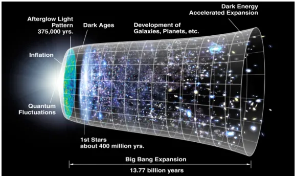
Expanding universe
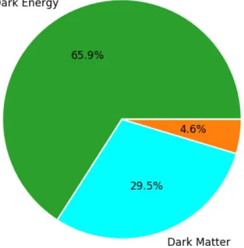
Dark matter
Dark energy
As shown in 1.3, DE has a negative pressure that distinguishes it from other types of matter such as radiation and baryons, which are also components of the universe. Understanding dark energy and devising solutions to the many related problems remains one of the most challenging issues in modern cosmology. In the next section we will introduce and derive some of the Friedman equations and their solutions in the framework of standard cosmology.
At the expansion factor z ~ 1010 this leads to a successful rendering of the origin of the light elements. We begin first by deriving a non-relativistic equivalent of the Friedmann equation from Newton's law of gravity and the second law of motion. From the gravitational acceleration on the outside of the sphere we can work out the equation of motion for Rs(t).
By multiplying both sides of (2.2) by dRs/d and integrating, we obtain the energy equation. where U is just an integration constant, which we define physically as the total energy per unit mass at the surface of the expanding sphere, that is, the sum of the gravitational potential energy and the kinetic energy per unit mass. 4Moving distance ignores the expansion of the universe, giving distance that does not vary in time.
Critical density and the density parameter, Ω
Since ρ(t) is proportional to 1/a3(t), we can see that ifU<0, the right-hand side of Eq. 2.7) will eventually reach zero after the expansion returns. Ω < 1, then it will always be less than unity because the sign on the right side cannot change [1].
The fluid equation
In solving the fluid equation, we require an additional equation of state that relates and P. Suppose we write this equation as P=wρ, where it may vary with time, but we will assume that its time derivatives are insignificant in comparison with the time derivatives of the densityρ.
The acceleration equation
Closed, open and flat universes
The density of the universe should be greater than the critical densityρ>ρc. On the other hand, an open universe means that gravity would be too weak to stop the expansion, which means it would expand forever. For a flat universe, the density is equal to the critical value; consequently, the universe will begin to contract only after infinite time.
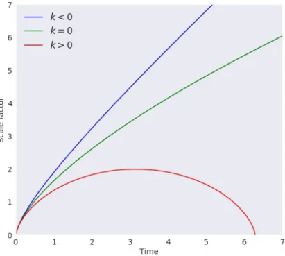
Solutions of the Friedmann equations
- Matter dominated universe (non-relativistic)
- Radiation dominated universe
- Matter dominated universe
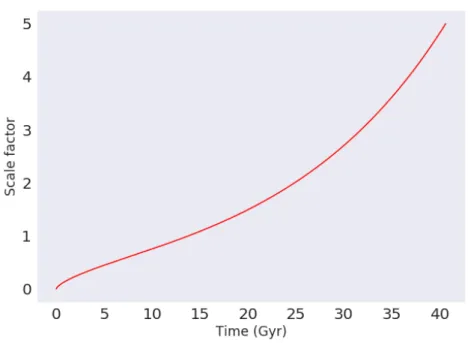
- Dark energy dominated universe
For dark energy, the equation of state is P = -ρ, then from the fluid equation we have
Solution of the Friedmann equation with total density
In the next chapter, we will present a useful technique in dynamical systems, which we will use to investigate a generalized system of Friedmann equations. The most commonly studied cosmological models have a system of autonomous ordinary differential equations (ODEs) as governing equations [28]. A brief introduction to what dynamical systems are will be given in the next subsection.
A dynamical system can generally be thought of as any abstract system consisting of a space (phase space or state space) and a mathematical law that relates the evolution of any point in that space. The state of the system we are interested in is represented by a set of critical system parameters; and the state space is the collection of all possible values for these parameters. Continuous dynamical systems are defined by a set of ODEs, while discrete-time systems are defined by differential equations or a map [29].
In this context, we are only interested in the type of dynamical systems that are continuous, as we investigate Friedmann equations, which for an isotropic and homogeneous space result in a system of ODEs. One of the methods that can be used to investigate properties of the stability of equilibrium points is the linear stability theory. To better explain this theory, we consider a mechanical system in one dimension F(x) =mx¨where Fi is a force.
Since in this text we aim to work with a system in two dimensions, we consider an autonomous system. The critical points can be distinguished using the following classification: If the resulting eigenvalues have negative real parts, then this point can be considered stable. If at least one of the eigenvalues has a real part that is positive, then the critical point involved would be unstable and thus correlate with a saddle point, which attracts and repels orbits in some directions.
Finally, the eigenvalues could all have positive real parts, where the critical point would be considered unstable and the trajectories repel [29]. In table 1 we present all possible cases for an autonomous system in two dimensions as equations 3.3. The exact same technique described above can be used when analyzing arbitrary dynamical systems, as a result we will use it in the context of cosmology to perform our analysis.
Defining parameters
The dimensionless variable m2 is important for the early evolution of the universe, but otherwise has a negligible value. In the next section, we look at different conditions of the Q interaction to explore the most likely form of interaction between dark matter and dark energy; and present the results. In this chapter, we therefore take a deeper look at the evolution equations by exploring some possible models of interactions between dark matter and dark energy.
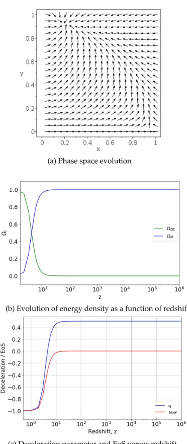
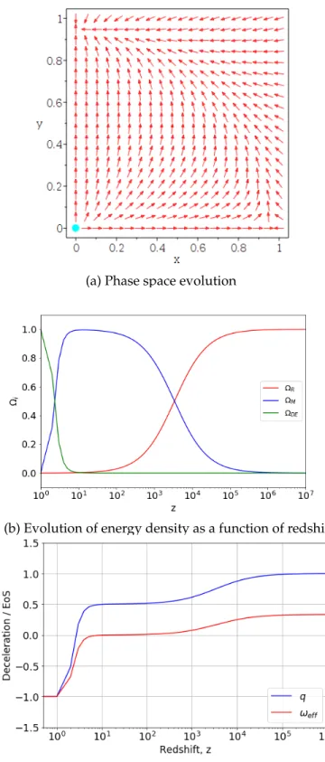
This point describes the early stages of the universe, meaning that matter and the late dark energy did not contribute to the energy content of the universe. Both the eigenvalues of the linearization matrix λ1 = 1/2 and λ2 = 1 are positive, demonstrating the instability of this phase. From this point we can deduce that this illustrates the age of dark matter in the universe, which is actually the matter-dominated phase.
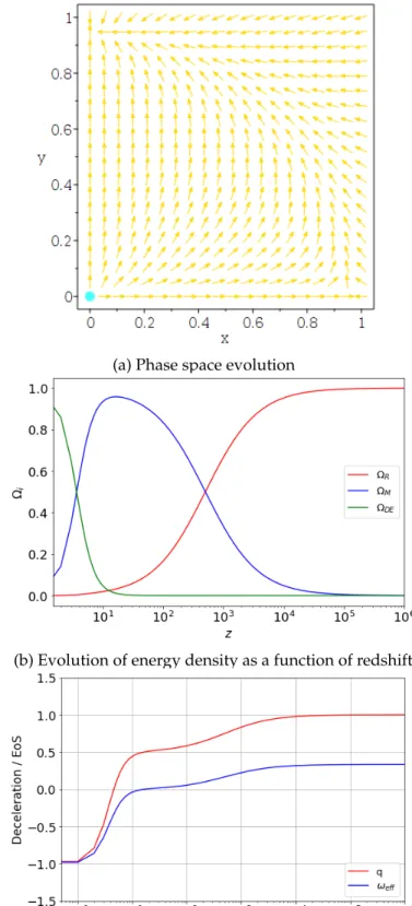
Since the constant m2 is small at late times, this critical point demonstrates a dark energy-dominated epoch of the universe. Because this point is too messy to include in this text, it is omitted, but upon checking it also showed trends of the dark energy period. Furthermore, the eigenvalues λ1 = 1 and λ2 ~ 1/2 are both positive, thus confirming the instability of the radiation era.
Since the eigenvalues λ1=−1 and λ2 ∼3/4 are positive and negative, the instability of the matter-dominated epoch is confirmed. The possible cause and commonality around these models is their linearity and inability to represent the radiation age in the early times of the universe. Dynamical systems were used to investigate the impact of interactions between dark matter and dark energy on the evolution of the universe.
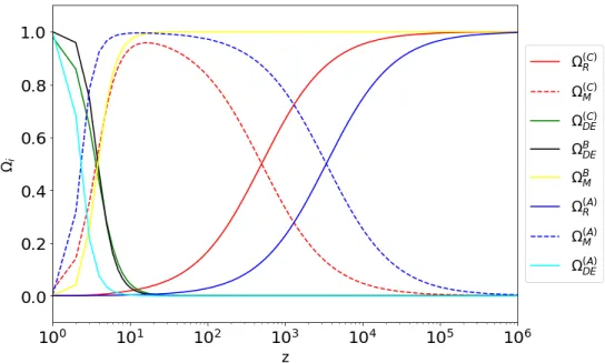
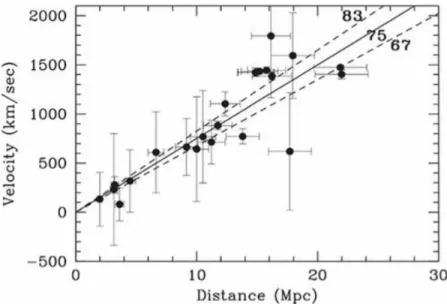
In the first chapter of this work, an introduction to the expansion of the universe was presented. It has been said that since the discovery of the current accelerating expansion of the universe in 1998, dark energy has played an important role in cosmological studies [40]. However, there were several interaction terms (B, E, H, and J) between DM and DE that we observed decaying a system at early times of the universe (the 3.26 system was divergent), and thus they only exhibited trajectories that started from the age dominated by matter to the age dominated by dark energy.
To ensure the stability of the models studied, we placed constraints on the coupling constant b2, which allowed us to constrain the effective EoS for dark energy. Iqbalet al., “Advances in cosmic physics,” International Journal of Astronomy and Astrophysics, vol.
![Figure 4: Possible geometries of the universe represented by the curvature index k. Credit: [2].](https://thumb-ap.123doks.com/thumbv2/pubpdfnet/10398238.0/18.918.160.771.701.883/figure-possible-geometries-universe-represented-curvature-index-credit.webp)