One of the most important steps in this process is the calculation of cooling loads. The cooling load was estimated for each of the buildings connected to the district cooling system. The capital and operating costs of the district cooling system and a more traditional system were compared.
ESTIMATES OF OVERALL COOLING LOADS 152
CUMULATIVE CHILLED WATER FLOW RATES THROUGH
ESTIMATE OF THE CAPITAL COST TO CONSTRUCT A
Mlaherbe Library 64 Figure 6.4 (a) - (f) Cooling load results for the Business Concourse 65 Figure 6.5 (a) - (f) Cooling load results for the New Chemistry Laboratory 66 Figure 6.6 (a) - (f) Cooling load results for the building of Chemical Technology 67 Figure 6.7 Cooling load for the district cooling system 68 Figure 7.1 Thermocline height as a time fiction for February 73.
LIST OF TABLES
INTRODUCTION
This report deals primarily with the energy consumption (and the financial costs thereof) associated with comfort air conditioning systems. These factors vary from country to country, but the main concern used to be the provision of comfortable internal environments at the lowest cost. This means that the provision of a pleasant internal environment should not detract from the focus of an institution's main activity.
LITERATURE SURVEY
The vapour compression cycle
Deviation from constant entropy lines is based on compressor efficiency. In order to obtain the capacity of the machine in energy units such as kW (kJ/s), the specific cooling effect must be multiplied by the mass flow rate of the refrigerant through the evaporator. In the simple vapor compression cycle shown in Figures 2.1 and 2.2, the mass flow rate is constant throughout the cycle. Refrigeration equipment can be compared based on the amount of energy required to achieve a certain amount of cooling.
![Figure 2.2: The theoretical single-stage vapour compression cycle, courtesy of Parsons [20]](https://thumb-ap.123doks.com/thumbv2/pubpdfnet/10637427.0/22.849.161.723.424.839/figure-theoretical-single-stage-vapour-compression-courtesy-parsons.webp)
ELECTRICITY GENERATION IN SOUTH AFRICA
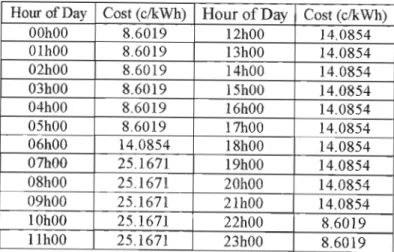
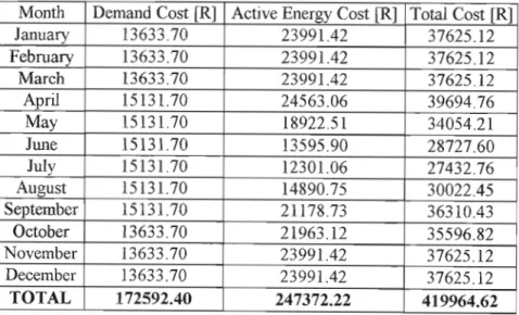
The total cost to the user consists of the demand cost (demand charge multiplied by maximum demand for the month) and the active energy cost (active energy charge multiplied by the energy consumption for the month). Sensible heat transfer to a room results in a change in the temperature of the air in that room. A latent heat increase implies an increase in the moisture content of the air in the room.
COMPUTER SIMULATION OF COOLING LOADS
LOADEST
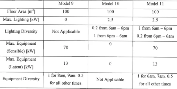
Some of the required attributes include floor area, wall and window areas, internal heat sources such as lighting and equipment, and details of human employment. At this stage it is possible to display the cooling load profile for each zone, but it is usually more interesting to see the simultaneous heating load profile for many zones (all served by a single air handling unit).
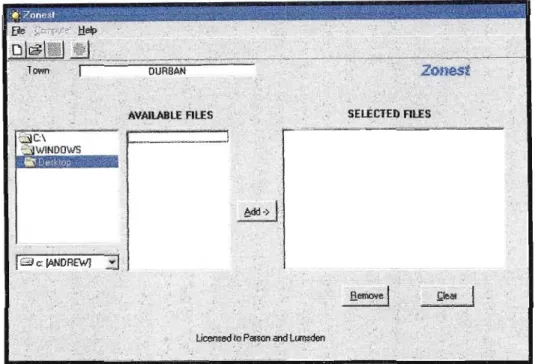
ZONEST
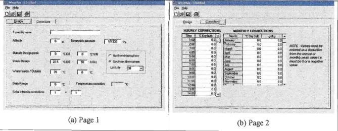
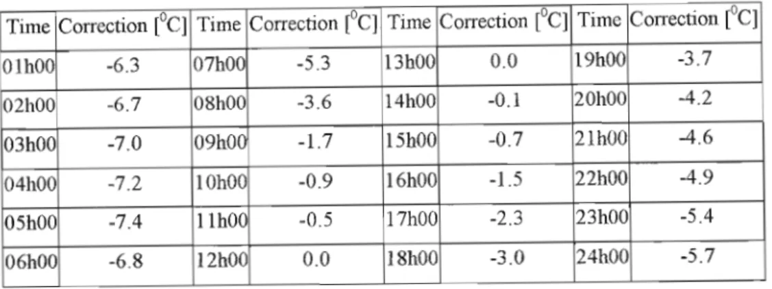
This allows the user to construct a profile of the temperature/humidity relationship for each month of the year. The moisture ratio corrections are shown in Table 4.3 for each month, in units of g/kg. The corrected values of the humidity ratio are shown in Table 4.4 for each month, in units of glkg.
The user interface of LOADEST
- LOADEST
- ZONEST
- The WEATHER UTILITY
However, in the second method, the accuracy of the cooling load due to each source can be validated one by one. Three models were used to validate the accuracy of LOADEST in determining the cooling load due to these heat sources. The cooling load caused by the residents depends only on the internal dry bulb temperature and the degree of activity.
CLTD = (A)(U)
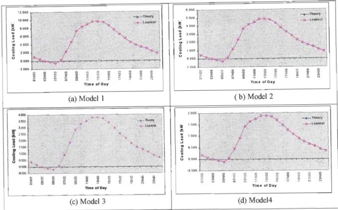
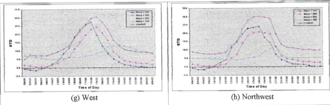
It was decided not to validate the accuracy of LOADEST by calculating only the cooling load, but instead to compare the CLTD values used. Second, the LOADEST cooling load value is almost always higher than any of the theoretical curves. It was found that there is no constant factor relating the LOADEST curve to any of the theoretical curves.
This could be detrimental to the design, as underpowered equipment may be supplied if the cooling load due to solar gain is a large percentage of the total cooling load. Each of the four graphs shows an approximation of the BEST LOAD and actual conditions for one month. There is almost exact agreement between LOADEST and theory for many cooling load sources.
The heart of the current system is a cold water tank located in front of Roward College. Under this definition, UND's campus cooling arrangement constitutes a district cooling system. During the charging cycle, the required water is pumped pmnp, via the main chilled water pumps 1 and 2, from the top of the tank to the cooler.
Wann water is pumped from the top of the storage tank to the chillers in the Denis Shepstone building by means of two primary chilled water pumps.
COOLING LOAD ESTIMATES FOR THE UND CAMPUS (USING LOADEST SOFTWARE)
Cooling load estimates for Howard College
Cooling load estimates for the Business Concourse
OPERATION, PERFORMANCE AND COST ANALYSIS OF THE UND DISTRICT COOLING SYSTEM
Total pipeline loss
The total pipeline loss (as considered in this study) is the sum of the losses due to friction, and those due to fittings.
Power requirements of pipelines
The power calculated from (7-3) is the amount of power required to transport the liquid through the pipe. The power drawn by each pump is the required power divided by the efficiency of the pump. The efficiency of each secondary chilled water pump was assumed constant because each is equipped with a variable speed drive to maintain efficiency close to peak design values.
8.0 CIl ~ 6.0
In 7.4.5 it was found that the energy consumption of secondary chilled water pumps can be neglected. For the same reasons, the energy consumption of primary chilled water pumps will also be neglected. The energy consumption of cooling devices represents the majority of the electrical consumption of the district cooling system.
No information was provided regarding the power factor of chillers currently installed on campus. Another cost to consider is that of servicing and maintaining equipment associated with the district's cooling system. Information regarding the maintenance cost for the three chillers and pump equipment was obtained from FMG, the facility managers entrusted with the operation of the district's cooling system.
This chapter covers most of the important aspects regarding the district cooling system on the UN campus. By the way, in practice the coordinators of the district cooling system [md that a total of 31 cooling hours is usually sufficient to provide adequate cooling in the summer. The operating cost of the system is a sum of the cooling cost and the maintenance cost, both of which have been calculated.
The aim is to contrast the two types of systems so that the economic benefit of the district cooling system (if any) can be quantified.
PROPOSAL FOR INDIVIDUAL CHILLER UNITS
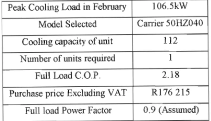
The Business Concourse
The following data applicable to the selection of the refrigeration equipment for The Business Concourse are solarized in Table 8.4 and Figure 8.4. The data relevant to the selection of the refrigeration equipment for the new chemistry laboratory are summarized in Table 8.5. The following data applicable to the selection of cooling equipment for the offices in the Chemistry Building are summarized in table 8.6.
A similar method was used to calculate operating costs for each of the refrigeration equipment selected earlier in this chapter. Operating costs are a function of cooling load and equipment characteristics and are summarized in Tables 8.7 through 8.9 and Figure 8.5. It was mentioned that the district cooling system chillers are almost always operating at full load. The result is that C.O.P.
The total cooling cost is simply the sum of the demand and active energy costs, which were found in 8.7.1 and 8.7.2 respectively. The subject of maintenance costs was briefly discussed in 7.8 with respect to the district cooling system. The only capital costs found to be specific to this type of refrigeration were the costs of the equipment itself.
The simple payback period result seems quite attractive, suggesting that the capital expenditure can be recovered within ten years.
Life cycle cost analysis
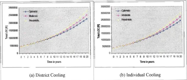
Cooling and maintenance costs for each of the 20 theoretical years were based on current costs and adjusted using the following equation; The total LCC can be more effectively compared for each of the three economic scenarios in Figure 9.3. In Figure 9.3, however, no correction of the value of the equipment was taken into account at any stage during the 20-year operating period.
It was concluded that (neglecting salvage values) the circuit cooling system is economically preferable to the individual cooling system because the total LCC benefits are recognized within the expected useful life of the equipment. TIlis analysis was then adjusted to reflect the salvage value of the equipment at any given time within the 20-year period. It can be seen that the total LCC curve for the circuit cooling system always lies below that of the individual cooling option.
The total LCC cost situation in the last example is best reflected by the graphs in Figure 9.3 which clearly illustrate the differences in capital cost, the effect of increases in operating costs and the point at which the total LCC for a system begins to increase above that of the other. . One of the uses of all these factors has been turbulence in the field of exchange rates, as shown in figure 9.5. a) Rand-dollar exchange rate Cb) Euro-dollar exchange rate. It is therefore important for one to understand that the merit of a zone cooling system cannot be judged on a "one time" basis.
If exchange rates continue to fluctuate widely, or if suitable equipment becomes available at favorable rates, then the economic viability of the district cooling system will change.
CONCLUSIONS
It was found that the district cooling system meets the goal of reducing cooling costs. The conventional cooling system (whereby each building would contain equipment to meet only its own cooling load) was found to require lower capital costs. The payback period (apart from the interest) for the district cooling system is approximately 9 years (figure 9.1).
Another method (total LCC) was also used to determine whether a district cooling system is economically advantageous compared to a conventional cooling system. It was found that the total LCC cost of a district cooling system would be lower than the cost of a conventional system after only 7 years, if the values of the used equipment were neglected. Therefore, it was concluded that a district cooling system would be economically superior to a conventional cooling system if a new cooling system was required for the 6 buildings in this study.
This is because total LCC savings would be realized within the economic life of the equipment lmder consideration. Considering the salvage value of the cooling equipment during total LCC analysis showed that the total LCC for the district cooling system would always be lower than that of a conventional cooling system. Current exchange rates (Rand vs Dollar and Dollar vs Euro) seem to have affected the total LCC of each system.
It was concluded that the economic viability of a district cooling system is influenced by exchange rates and the choice of equipment supplier.
APPENDICES
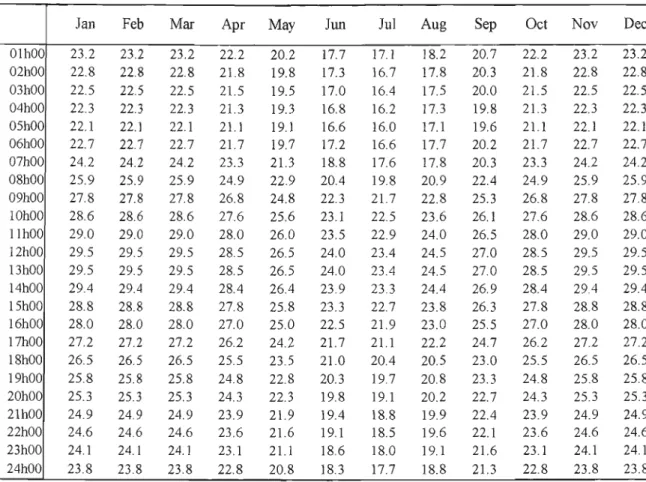
DURBAN TEMPERATURES
జాన్ ఫేబ్ మార్ ఏపే మేజ్ జూన్ జుల్ ఆగస్టు సేఫ్ యాక్ట్ నవంబర్ డెక్ జాన్ ఫేబ్ మార్ ఏప్ ఎంఎం.
COOLING LOAD ESTIMATES ASSUMING FULL VENTILATION
COOLING LOAD ESTIMATES ASSUMING ZERO VENTILATION
COOLING LOAD ESTIMATES TAKING INTO ACCOUNT VENTILATION DIVERSITY
ESTIMATES OF INSTANTANEOUS COOLING LOADS
02hOO 03hOO
23hOO 24hOO
24hOO
19hOO 20hOO
20hOO 21hOO
19hOQ 20hOO
ESTIMATES ON PULL-DOWN COOLING LOADS
09hOO 10hOO
03hOO 04hOO
0.002hOO
TOTAL
08hOO 09hOO
ESTIMATES OF OVERALL COOLING LOADS
01hOO 02hOO
CUMULATIVE CHILLED WATER FLOW RATES THROUGH THE THREE SECONDARY CHILLED WATER PUMPS
TOTAL LIFE CYCLE COSTING DATA
![Figure 2.4: C.O.P. as a percentage of full load C.O.P. for various chiller types, derived from EPRI [6]](https://thumb-ap.123doks.com/thumbv2/pubpdfnet/10637427.0/28.856.143.754.109.460/figure-percentage-load-various-chiller-types-derived-epri.webp)
![Figure 2.6: Basic stratified chilled water configuration, courtesy of Dorgan & Elleson [9]](https://thumb-ap.123doks.com/thumbv2/pubpdfnet/10637427.0/34.853.240.654.157.579/figure-basic-stratified-chilled-configuration-courtesy-dorgan-elleson.webp)
![Figure 2.8: Typical temperature distribution in a stratified thennal storage tank, courtesy of Dorgan & Elleson [9]](https://thumb-ap.123doks.com/thumbv2/pubpdfnet/10637427.0/35.846.200.687.106.438/figure-typical-temperature-distribution-stratified-thennal-courtesy-elleson.webp)
![Figure 3.1: Illustration of the heat storage phenomenon for light, medium and heavy construction, courtesy of McQuiston and Parker [4]](https://thumb-ap.123doks.com/thumbv2/pubpdfnet/10637427.0/39.846.153.725.113.370/figure-illustration-storage-phenomenon-construction-courtesy-mcquiston-parker.webp)