Graph reduction techniques for exergy-based FDI on the Tennessee Eastman process

Three FDI methods are applied to the GTLP graph data to generate a control data set. As an example, Figure 1.2 [6] shows the composition of the attributed graph of a coal-fired power plant.

Figure 1.1: Categories of fault diagnostic methods [3].

Problem statement

Research objectives

Formulate graph reduction techniques
Generate the FDI control data set
Develop an experimental design
Evaluate the graph reduction techniques on an additional process

To evaluate the efficiency of the proposed graph reduction techniques, the performance of the FDI methods is first determined using standard, unreduced graph data attributed to the benchmark process. To validate this study, it is necessary to show that graph reduction is a general solution that is not only valid when applied to the attributed graph data of a specific process.

Methodology

Formulate graph reduction techniques
Generate the FDI control data set
Develop an experimental design
Evaluate the graph reduction techniques on an additional process

Once the imputed graph data has been processed to a format compatible with the FDI methods in MATLAB®, each FDI method is applied to the graph data. All three FDI methods are first applied to the unreduced imputed graph data of the GTLP, and the performance of each FDI method is used as a set of control data.

Figure 1.3: Logic flow diagram of the experimental process applied to the graph reduction techniques in this study.

Dissertation outline

To evaluate the effect of the graph reduction techniques on the attributed graph data of the GTLP, a procedure similar to that used for the TEP graph data is followed. Subsequently, the experimental process from the previous chapter is repeated on the GTLP to determine the effectiveness of the reduction techniques on the GTLP.

Energy visualisation

Energy

Exergy

Comparison of energy-based and exergy-based methods

Graphs

Attributed graphs
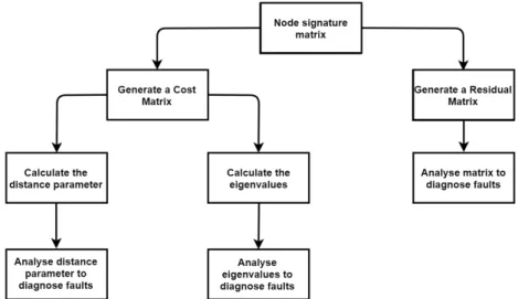
Graph comparison for FDI
Graph comparison by generating a cost matrix
Graph comparison by generating a residual matrix

In [7], cost matrices are also developed by comparing the NSM of the system in NOC with the NSM of each fault condition. An operational cost matrix can then be developed by comparing the operational NSM with the NSM of the system in NOC.

Graph reduction

Graph reduction through graph summarization

Structural graph summarization
Attribute-based summarization
Hybrid graph summarization
Using a summarized graph for FDI

The k-SNAP operation also allows the user to determine the size of the resulting digest. The CANAL technique automatically categorizes the numerical values by assessing the similarities of the attribute values and link structure of all nodes in the graph.

Figure 2.4: Graph summarization process [27].

Graph reduction through attribute filtering

Using a graph reduced with attribute filtering for FDI

The reduced graph with unchanged attributes is compared with itself under NOC and a cost matrix is generated. During plant operation, the attributes of the reduced graph are constantly monitored and updated by taking plant measurements.

Summary of graph reduction methods found in literature

The eigenvectors and eigenvalues of this cost matrix are calculated and compared to those of normal plant operation to determine whether a failure has occurred. Ideal for graphs with numeric attributes and it is possible to verify the size of the summarized graph.

Benchmark model - Tennessee Eastman process

Tennessee Eastman process

The products leaving the reactor are in vapor form and are condensed by the product condenser before going to the vapor-liquid separator. With advances in computer systems, it has become increasingly popular to use data-driven schemes for TEP.

Critical literature review

When reviewing the various techniques available for data reduction of an attributed graph, it is essential to consider the effect each technique has on the structural information contained in the attributed graph. Comparing graph reduction with attribute filtering and graph reduction with summarization as discussed in this section (see Table 2.2), it is clear that graph reduction with attribute filtering is better at preserving rather than distorting structural information, since the nodes of the original graph are not joined . into supernodes.

TEP model overview

This chapter reviews specific literature related to the exergy characterization of the TEP model and the development of its ascribed graph. The comparison performed during each step indicates that the results obtained from the Simulink® model and the results obtained from the FORTRAN code have a reasonable correlation.

Fault conditions

The second step involves comparing the closed-loop TEP Simulink® simulation results with the results produced by simulating the TEP with the results from the FORTRAN code used by [44].

Calculating exergy attributes

Linear regression analysis produced an equation for the standard chemical exergy of substances in the vapor phase [12], which is expressed as. Linear regression analysis again produced an equation for the standard chemical exergy of TEP substances in the liquid phase [12], which is expressed as.

Attributed graph of the TEP

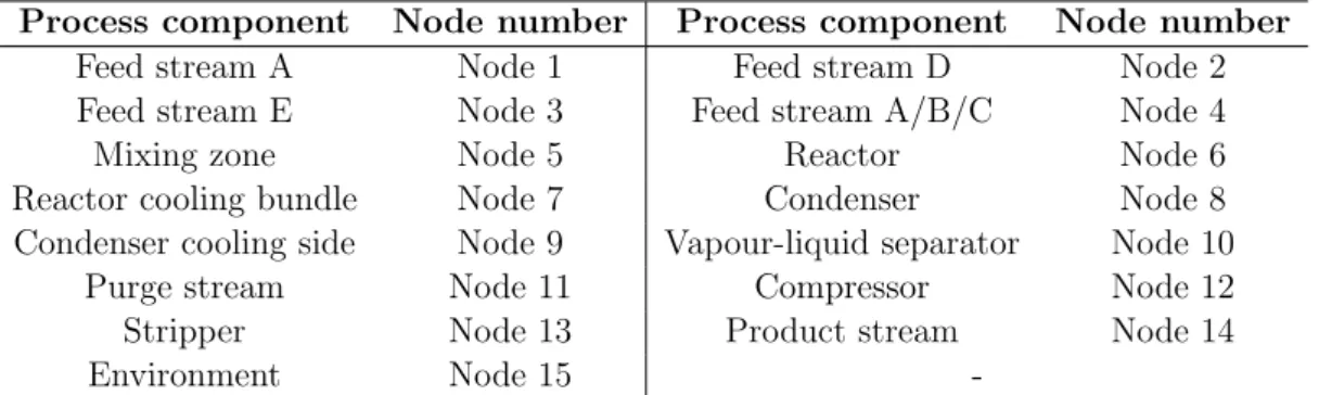
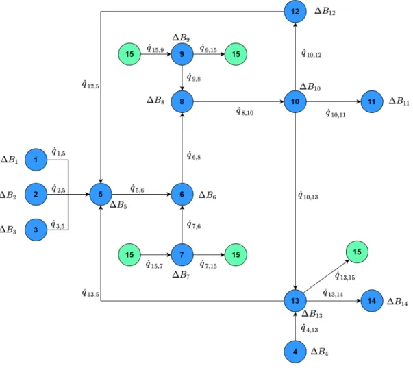
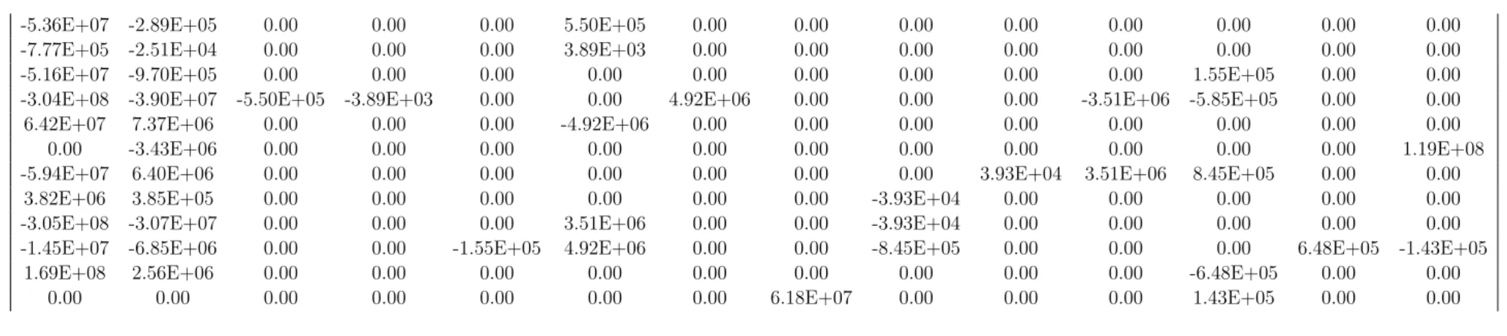
The NSM of the imputed graph of the TEP, as illustrated in Figure 3.2, can be expressed as. Because links are directional; the link attribute is multiplied by −1 when the link is inverted.

Conclusion

The diagonal entries of the connectivity attribute matrix are all zeros, seeing that no node is connected to itself. This chapter provides a broad overview of the methodology used to implement each of these three FDI schemes.

Generating control data for FDI schemes

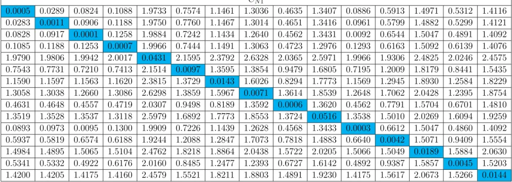
Generating a cost matrix

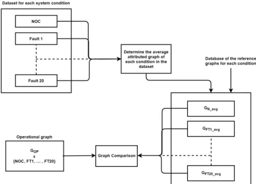
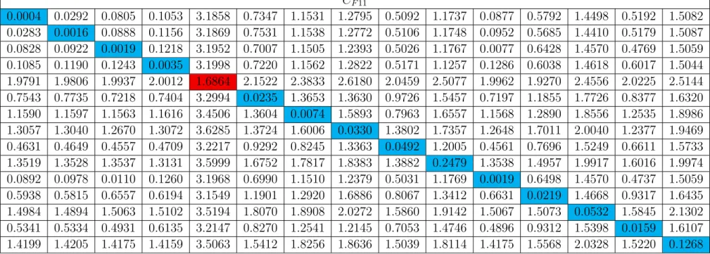
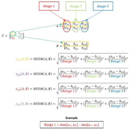
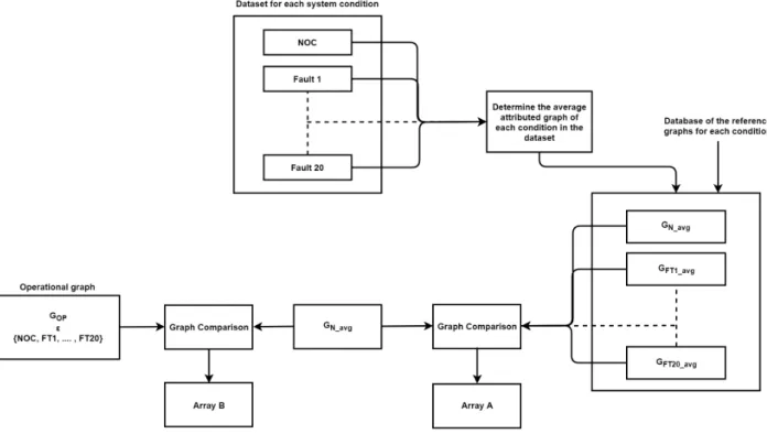
The operational attributed graph is then compared to each reference attributed graph, creating a cost matrix. One sample operational attributed graph under NOC is compared to a normal reference attributed graph to produce a specific cost matrix.

Figure 4.3: Illustration of the cost matrix generation process.

Distance parameter method

Detection
Isolation

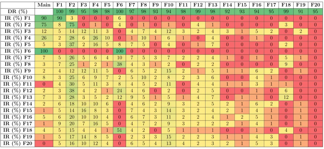
It is clear from Figure 4.7 that the distance parameters produced by comparing the operational attributed graphs of Fault 2 with the reference attributed graph of Fault 2 are for the most part smaller than any of the other distance parameters. Most of the time, the distance parameters produced by comparing the operational attributed graphs of Error 8 to the reference attributed graph of Error 8 are not smaller than any of the other distance parameters.

Figure 4.6: Illustration of how the distance array is produced from the array of cost matrices.

Eigendecomposition method

Detection
Isolation

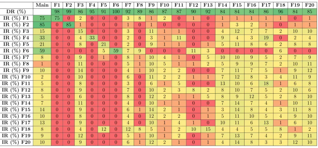
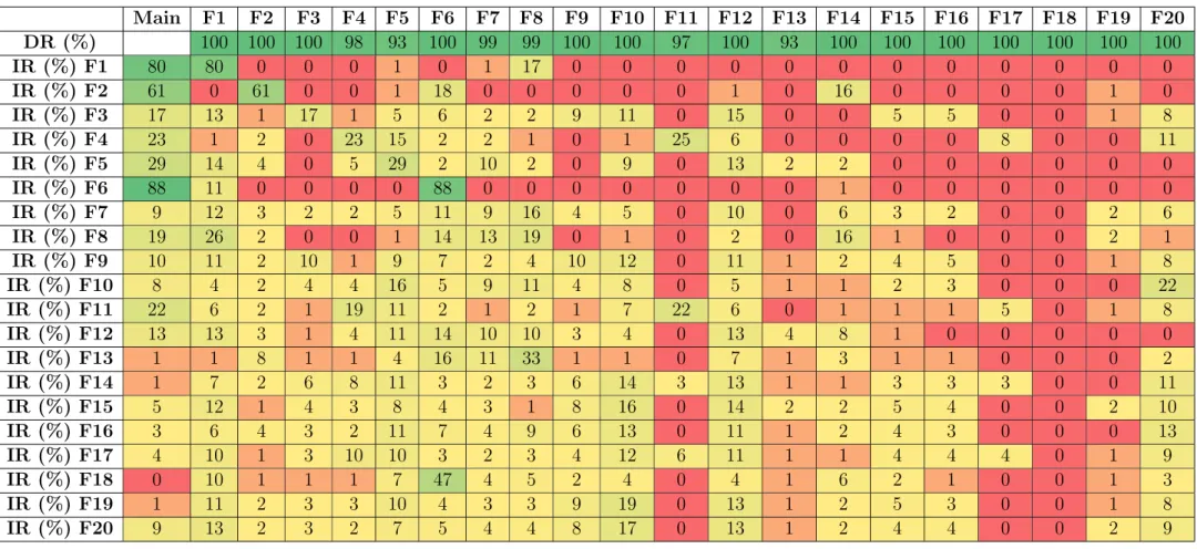
To determine the total insulation percentage of this FDI method, the diagonal entry of the insulation percentage rows in Table 4.3 is taken into account. To determine the total insulation percentage of this FDI method, the diagonal data of the insulation percentage rows of Table 4.6 are again considered.

Figure 4.9: Illustration of the graph comparison operation for the eigendecomposition method.

Modified eigendecomposition FDI method

The overall isolation rate for the eigendecomposition FDI method applied to the TEP data is calculated to be 17.80. The confusion matrix and the specific detection and isolation rates of the modified self-degradation FDI method can be found in Tables 4.9 & 4.10 respectively.

Residual-based method

Detection
Isolation

The residual matrix generated by comparing the operational attributed graph of the system in NOC to the reference normal attributed graph should theoretically be zero. FDI method, the reference attributed graph of each condition is also the average of the 501 operational attributed graphs of that condition.

Table 4.10: Detection and isolation rates of the modified eigendecomposition method.

Summary of results

If a choice had to be made, the self-degradation method would be chosen as its overall detection and isolation rates are slightly lower than the residue-based FDI method and it is the best performer in terms of specific isolation rates. These results (Table 4.14) now serve as a set of control data against which the results of the FDI schemes using the reduced allocated graphs can be compared.

Conclusion

This chapter describes graph reduction techniques that have been proposed as potentially viable options for reducing the size of the attributed graph data used in graph-based FDI methods. Guidelines on how the results of the experimental process should be interpreted are also discussed.

Table 4.13: Detection and isolation rates of the residual-based FDI method.

Proposed graph reduction techniques

Link attribute reduction techniques and node attribute reduction techniques reduce the complexity of the attributed graph in different ways. Link attribute reduction techniques reduce complexity by zeroing specific attribute values in the NSM, which means that the mathematical operations of the FDI methods evaluate fewer attributes.

Table 5.1: Summary of the graph reduction techniques proposed in this study.

Experimental design

Overview

Technique # FDI Method Reduction Interval Measured Performance Indicator Technique 1 Distance 10th percentile Overall Detection Rate (%) Technique 1 Distance 10th percentile Overall Isolation Rate (%) Technique 1 Distance 10th percentile Attributes reduced non-zeros (%) Technique Specification 10th percentile isolation rate 1 (%) Technique 1 Distance 10th percentile Specific isolation rate 2 (%) Technique 1 Distance 10th percentile Specific isolation rate 3 (%) Technique 1 Eigen 10th percentile Overall detection rate (%) Technique 1 overall isolation percentile 10th %) Technique 1 Eigen 10th percentile Reduced non-zero attributes (%) Technique 1 Eigen 10th percentile of Specific isolation rate 1 (%) Technique 1 Eigen 10th percentage Specific isolation rate 2 (%) Technique 1 Eigen 10th percentile Specific3 ) Technique 1 Residual percentage 10th Overall detection rate (% ) Technique 1 10th Percent Residual General Isolation Rate (%) Technique 1 10th Percent Residual Reduced Nonzero Attributes (%) Technique 1 10th Percent Residual Specific Isolation Rate 1 (%) Residual 10th percent Specific isolation rate 2 (%) Technique 1 Residual 10th percent Specific isolation rate 3.

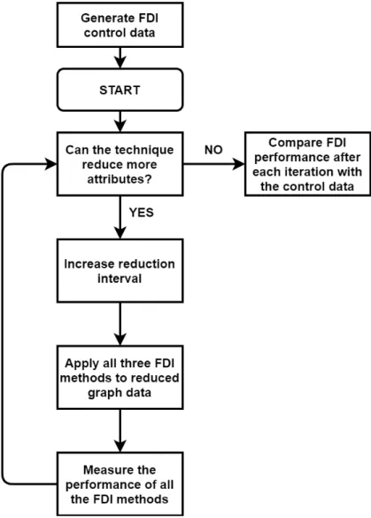
Analysis of the results

It is then possible to determine the trajectory of this change in performance, the reduction ranges at which the reduction techniques perform well, and which reduction techniques perform better than others.

Conclusion

In addition, it will also be possible to determine the extent to which each reduction technique can reduce the graph data before the performance of the FDI methods begins to degrade too much. The individual reduction techniques are also applied in various combinations to the assigned graph data to determine whether it is possible to overcome the shortcomings of the individual techniques.

Evaluating the graph reduction techniques

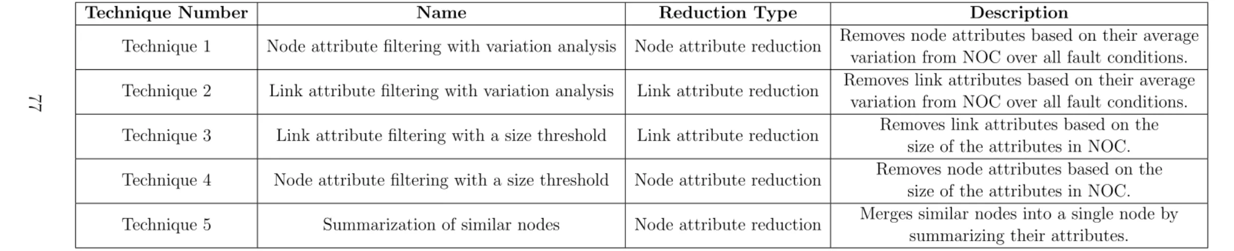
Node attribute filtering with variation analysis
Link attribute filtering with variation analysis
Link attribute filtering with a size threshold
Node attribute filtering with a size threshold
Summarization of similar nodes

The overall detection and isolation rates of the FDI methods relative to the percentage of attributes removed from the graph data are shown in Figures 6.9 and 6.10, respectively. The overall isolation rates of the three FDI methods also remained relatively stable as more attributes were reduced.

Figure 6.1: The overall detection rates after applying Tech- Tech-nique 1.

Interpretation of results

Such is the case with the specific insulation percentages of the remote FDI method, which are recorded in Table 6.1. For example, for the remote FDI method, techniques 1, 2, and 5 at specific thresholds were the most complementary reduction techniques when examining the performance of the FDI method after applying these techniques to the graph data.

Combining reduction techniques

Combining techniques for the distance FDI method

Moreover, when comparing these performance results with the results of the distance FDI method after applying the individual. The combined reduction technique proposed for the distance FDI method also significantly reduces the execution time of the FDI method.

Combining techniques for the eigendecomposition FDI method

The performance of the self-decomposition FDI method after applying the combined reduction technique can be seen in Table 6.8. The execution time of the method using graph data reduced by the combined technique is significantly lower.

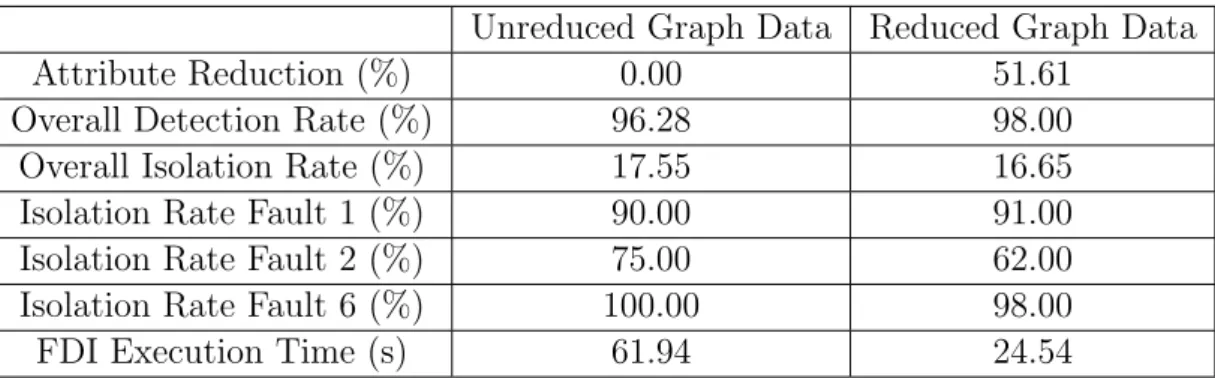
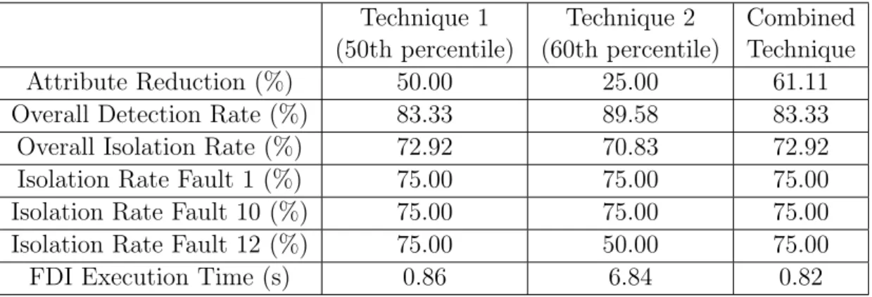
Table 6.8: Performance of the eigendecomposition FDI method after applying the combined reduction technique.

Combining techniques for the residual-based FDI method

A comparison of the performance of the residual-based FDI method using unreduced graph data and the performance of the method using graph data as reduced by this combined technique is shown in Table 6.10. The resulting imputed graph plot of the TEP after applying this combined technique is shown in Figure 6-13.

Table 6.10: Performance of the residual-based FDI method after applying the combined reduction technique.

Verification

Verification of Technique 1

During the verification of Technique 2, a discrepancy was noted between the MATLAB® scaled plot and the Excel® scaled plot. After correcting this, the MATLAB®-reduced graphs matched all the corresponding Excel®-reduced graphs.

Table 6.11: Reduced attributed graph produced by implementing Technique 1 in Excel.

Conclusion

Validation is performed by determining whether the graph reduction techniques proposed in this study are general solutions that can reduce the data in the graph while maintaining the same level of FDI performance regardless of the process used to generate the graph data. For this purpose, gas-to-liquid process graph data is generated and reduction techniques are applied to the data.

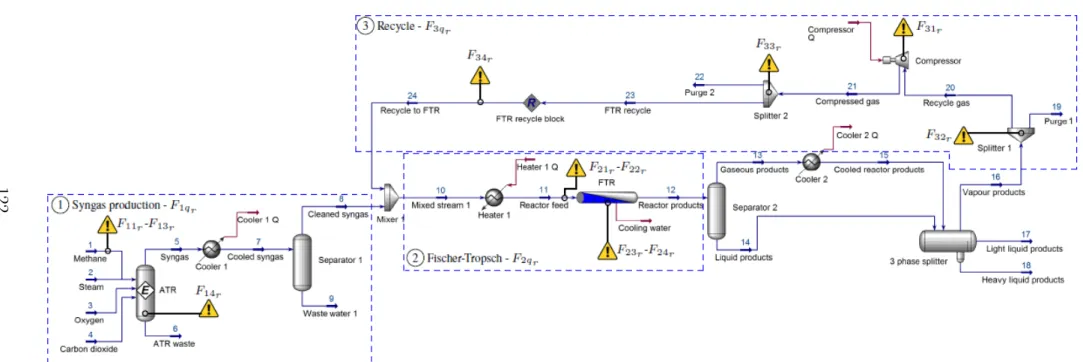
Gas-to-liquids process overview

Synthesis gas production

Pre-reforming is used to prevent the heavier hydrocarbon products from cracking in the first section [60]. After pre-reforming is applied, a reforming process, which is the primary mechanism for producing syngas, is used [8].

Fischer-Tropsch synthesis

Syngas, also referred to as syngas, is a mixture of hydrogen (H2) and carbon monoxide (CO) and chemical reforming is usually used to produce it. If necessary, the syngas can also undergo conditioning whereby aspects of the syngas, such as composition or temperature, are changed.

Product upgrading

In fractional refining, some products need to be refined and others must be mixed to obtain final products (intermediate and final). Finally, in self-refining, all products obtained are finished products (finished).

GTLP model overview

Modelling assumptions

Modelled process flow

Fault conditions

Selecting faults

Fault sets

Exergy-based graph of the GTLP

Applying the FDI methods to the GTLP

The attributed process graph in NOC remains the same, despite the different sizes. Any future reference to the self-decomposition FDI method refers to this modified version of the self-decomposition FDI method.

Figure 7.3: Illustration of fault locations within the GTLP.

Evaluating the graph reduction techniques on the GTLP graph data

The overall detection and overall isolation rates of each reduction technique with increasing reduction range can be seen in the figures below. Tables containing overall detection and overall isolation rates, as well as specific isolation rates for each reduction range of each reduction technique, can be found in Appendix E.

Observations from the results

The overall detection rates for all three FDI methods applied to the GTLP data remained relatively constant over most reduction intervals. It is further evident that the reduction techniques relying on attribute variation analysis (techniques 1 and 2) are effective when applied to the allocated graph data for both GTLP and TEP.

Applying combination reduction techniques to the GTLP

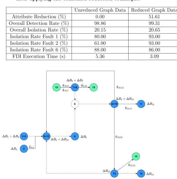
However, the evaluation showed that the performance of FDI resulting from individual complementary mitigation techniques can be improved by combining these techniques, although not in all cases. For the residual-based FDI method (Table 7.7), the combination of Technique 2 (60th percentile) and Technique 5 (1 merger) outperformed the individual mitigation techniques on every metric used for valuation.

Table 7.5: A comparative evaluation of combined reduction techniques for the distance parameter FDI method.

Validation

Although each proposed reduction technique did not affect the FDI methods in exactly the same way when different processes were used, for both TEP and GTLP, it was possible to formulate at least one reduction technique for each FDI method, resulting in similar FDI performance as is obtained before graph reduction. The concept of a general solution is further supported by the fact that the two processes differ significantly in terms of graph structure, error ratio and composition of graph data (dynamic vs steady-state system), as well as the fact that three different FDI methods were used for evaluation of the techniques.

Conclusion

It can therefore be concluded that graph reduction is a general solution and can be considered validated. Subsequently, the last part of this chapter contains several recommendations on how to use these results and findings in future work.

Concluding remarks

Some interesting observations can be made from the response performance of each FDI method to the reduction iterations of each reduction technique. First, the control data set was created by applying FDI methods to standard, unreduced imputed GTLP graph data.

Recommendations on future work

Kavuri, "A Review of Process Fault Detection and Diagnosis: Part I: Model-Based Quantitative Methods," Computers &. Vosloo, "Exergy-based fault detection and diagnosis of the Tennessee Eastman process", Doctor of Philosophy, North-West University, Potchefstroom, 2021.

Verification of Technique 3

Verification of Technique 4

Verification of Technique 5

Categories of fault diagnostic methods
Logic flow diagram of the experimental process applied to the graph reduction
Overview of the literature study with all the references used in this chapter
Example of a graph G
Graph summarization process
An example of structural graph summarization
Illustration of the SNAP operation
Example of hybrid graph summarization:(a) Original graph. (b) Summarized
Tennessee Eastman process model
Tennessee Eastman process model
Diagram of the attributed graph of the TEP
Process flow diagram of a graph-based FDI scheme
Illustration of how the FDI schemes use different graph comparison operations
Illustration of the cost matrix generation process
Illustration of how time-series data are used to perform graph comparison
Generating the cost matrices for an operational condition
Illustration of how the distance array is produced from the array of cost matrices. 49
Plot of distance parameters produced by comparing the operational attributed
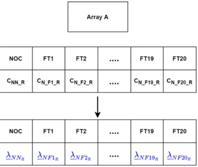
The array eigenvalues calculated from the cost matrices in array A
The array of eigenvalues calculated from the cost matrices in array B
Process flow diagram of the graph comparison operation used by the residual-
The array of frequency vectors resulting from the residual matrices in array A. 68
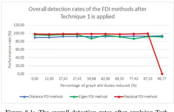
The overall detection rates after applying Technique 1
The overall isolation rates after applying Technique 1
The attributed graph diagram after applying the combined reduction technique
The attributed graph diagram after applying the combined reduction technique
The resulting attributed graph diagram after applying the combined reduction
The main processing sections of a GTLP
Simulation model of the GTLP as developed by Greyling in Aspen HYSYS ® . 118
Exergy-based attributed graph of the GTLP

This appendix contains the detection and isolation rates of all three FDI methods applied to the imputed graph data from the GTLP. Performance of the FDI methods using the GTLP graph data as reduced by all the reduction techniques.