Trajectory commands are sent from the base station to the robot via Wi-Fi for execution. In addition, the live video feed from the robot can be sent to the ground station's computer.
Nomenclature
J(¯twp),JP(¯twp) Trajectory cost function, and trajectory cost function with limit violation penalties, respectively. T Trajectory solver and control system time step size tC Time over which robot components consume charge.
Introduction
- Problem Statement
- Objectives
- Specifications
- Layout of the Dissertation
Obstacle avoidance was performed by simulating the robot's workspace environment and generating trajectories that allowed the robot to avoid obstacles in that environment. This dissertation has developed the robot's obstacle avoidance capabilities to a level where these trajectories can be generated autonomously, provided descriptions of the workspace obstacles have been provided to the simulator.
Literature Review and Background
Kinematics
- Forward kinematics
- Inverse kinematics
- Calculating the Jacobian
- Damped least squares
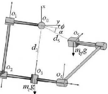
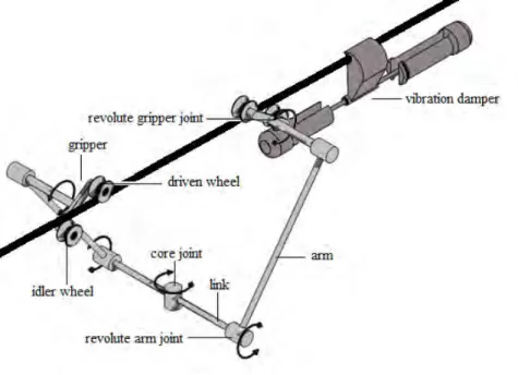
The robot can rotate around an axis from the transmission line coordinate frame O0. This applies to PLIR in cases where a specific target position (way point) for the end effector may not be achievable due to physical limitations of the robot.
Robot Modelling
- Inverse dynamics model
- Simulink model
The Simulink model was created by incorporating and modeling all the robot components at a basic level. The model parameters were then fine-tuned during comparison tests between the predicted and measured behavior of the robot.
Trajectories
- B-spline functions
- Fitting method
- B-spline order
- Time scaling
- Torque limiting
- Angular speed limiting
- Instantaneous current limiting
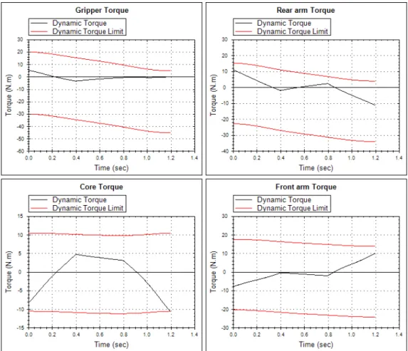
This is not the case with the PLIR where the dynamic torque limits change based on the position of the end effector. The torque plot in Figure 2.12 is a simulation output of the PLIR model discussed in Section 2.4.
Simulation
Limiting the robot's instantaneous power consumption is the simplest of the three constraints to deal with. Current limiting simply requires that the sum of the absolute values of all actuator currents at a given time not exceed this battery specification. This limit is to protect the battery and is unlikely to be reached during normal operation.
Obstacle avoidance
- Existing work
- Obstacle description
- Path planning
- Power line inspection robots
- Path planning implementation
The obstacles actually exist in the workspace and the representation of the obstacles in workspace makes visualization of the problem easier. This will help in developing the obstacle avoidance algorithms needed for the robot. The localization of the obstacles in the case of the PLIR is well known (connected to the line).
Based on the estimated state of the robot (position on the line and position relative to obstacles in the base), it combines basic motion elements to achieve obstacle avoidance. In the case of PLIR, such partial maneuvers are not suitable due to the configuration of the robot.
Trajectory optimisation
- Existing work
- Energy minimisation
- Time-energy minimisation
- Jerk minimisation
- Optimisation objectives
The minimization of the energy required by the trajectory with a given time interval is achieved by searching for the optimal maximum velocity of the trajectory along the path. With time-energy optimization, the cost function is a weighted sum of the total time taken for a trajectory and the total energy required for the trajectory. The cost function for the optimizer is described as the weighted sum of trajectory time and trajectory energy subject to constraints on velocity, acceleration, thrust, and torque.
It is the weighted sum of the rail time and the squared stroke time, subject to velocity, acceleration, and stroke constraints (similar to Saramago and Steffen (1998)). Due to the discrete nature of the cost trajectory solver, it cannot be computed in the federal time domain.
Obstacle Avoidance
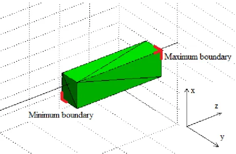
Axis-aligned bounding box description
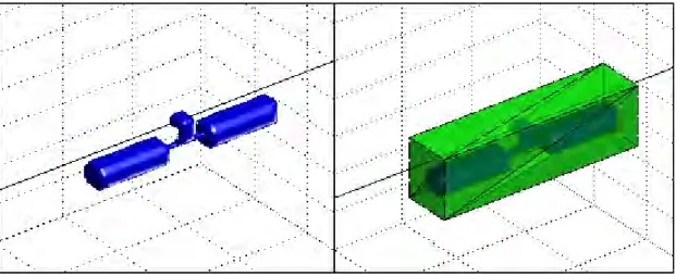
It can be used to model a complex obstacle that is relatively uniform along at least one axis, such as the z-axis (along the line) in the case of a vibration damping. For example, the vibration damper (modeled in relatively high detail in Section 2.3.2) can be modeled as an AABB. The dimensions and orientation of the box depend on the barrier itself, and these parameters are chosen in order to properly close the barrier.
In this case, AABB provides a sufficient description of the vibration damper to generate obstacle avoidance waypoints. A similar concept for this type of boundary description can be found in Schouwaarset al.(2001), section 3.
Implementation
- Waypoint selection
- Collision detection
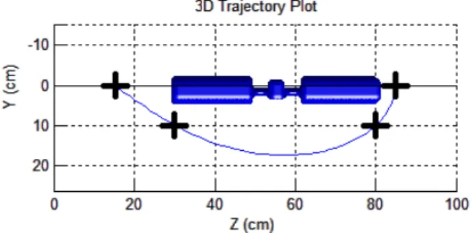
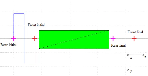
The simulated model has the robot stop 3 cm from the start of the obstacle presentation. The selection of waypoints is limited to a subset of the robot's workspace in the quadrant along the z-axis between the negative x-axis and the positive y-axis, as shown in Figure 3.9. The limitation is due to the physical configuration of the robot and the collision-free path-finding method used.
Since each of the robot parts is represented by a line segment, collisions can be investigated using the algorithm from Ericson (2005) that was used to perform line of sight checks. If any of the line segments that make up the robot cross an obstacle, a collision has occurred.
Trajectory Optimisation
- Time ratio optimisation
- Cost function analysis
- Implementation
- Optimisation performance
- Interval time optimisation
- Cost function analysis
- Implementation
- Optimisation performance
- Discussion and comparison
- TRO vs ITO
- ID model optimisation vs Simulink model optimisation
- Online vs offline optimisation
- Conclusion
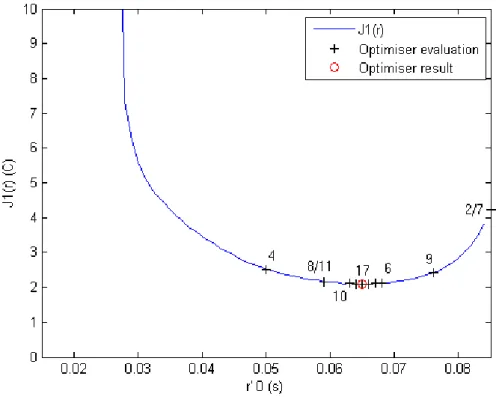
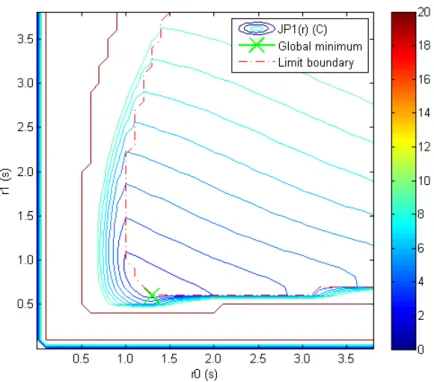
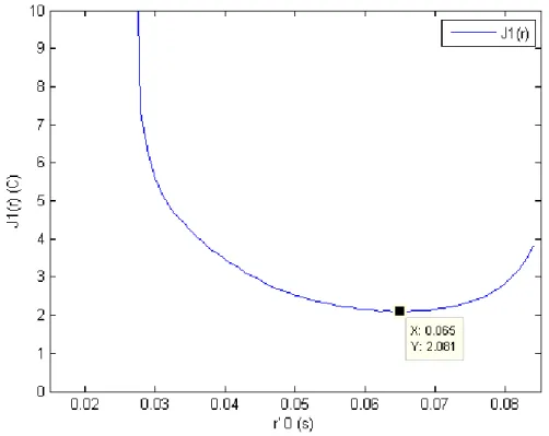
At the lower extreme ofr00 (Figure 4.1), the trajectory interval time allocated to the first part of the trajectory is only 15%. In this way, the behavior of the optimizer can be monitored as it tries to find the global minimum. The contour representation of the cost function of the model IDJ1P(¯r) for the trajectory~s1(¯θ(t)) is given in figure 4.6.
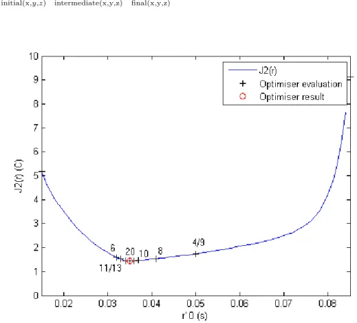
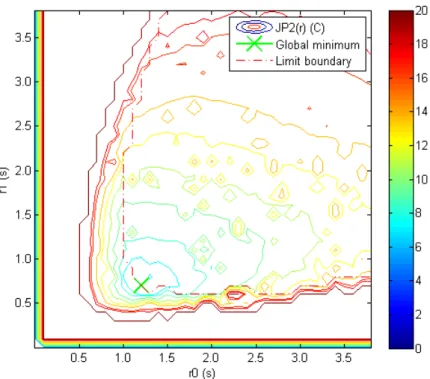
It shows the global minimum of the function J1P(¯r) as well as the torque/speed/current limit for trajectory~s1(¯θ(t)). The contour representation of the Simulink model cost function J2P(¯r) for trajectory ~s1(¯θ(t)) is given in Figure 4.7.
Implementation
PLIR Trajectory Solver
- Graphical user interface
- Code modules
- Inverse kinematics
- B-splines
- Inverse dynamics
- Simulink model
- Trajectory time scaling
- Obstacle avoidance
- Trajectory optimisation
- Trajectory simulation output
- Communication
- MATLAB integration
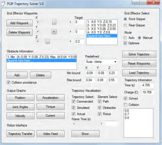
The "Path Visualization" group also allows the user to view a virtual presentation of the robot's maneuver. The trajectory simulation is animated when you open the window for the first time by clicking on “Show”. This section describes the functionality of each of the main code modules in the PLIR Trajectory Solver application.
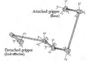
The Obstacles class provides the option to set the origin of the back clamp coordinate frame (i.e. the position of the front clamp) and retrieve the obstacle space information relative to this coordinate frame in order to create a trajectory and detect collisions as done for the forward trajectory. For the PLIR Trajectory Solver application, the functionality of interest is that of the Simulink environment.
PLIR on-board control software
- On-board PC software
- Microcontroller software
Autonomous control is used to execute the trajectories created by the PLIR Trajectory Solver application. The PLIR Interface application stores all the trajectory data regarding joint positions, speeds and current profiles. The data can then be imported into the PLIR Trajectory Solver application for analysis at a later stage.
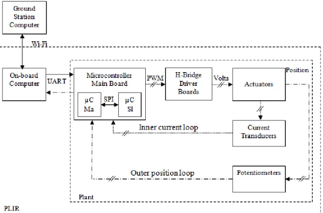
The master and the slave are each responsible for measuring and controlling the position and current of the drives connected to them. The slave sends its measurements to the master when it receives new commands from the on-board computer via the master.
PLIR control system
- Control system configuration
- Simulink model
- PID controller tuning
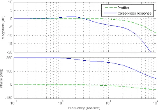
With the correct parameters, PLIR can be modeled using simple first-order transfer functions to describe the physical components of the system. A Bode plot of the open-loop plant transfer function (current command from the controller output) to the output (robot joint position) was created. The device in this case includes all components from the input of the main board of the microcontroller to the output of the position of the actuator, as shown in Figure 5.9.
Once the verified robot model is created, the linearized version can be used to tune the PID controller using the MATLAB SISOTool. The transfer function of the PID controller is given in serial form in (5.1) and is implemented in discrete time form on the robot computer.
Hardware
- Ground station computer
- PLIR computer
As shown in Figure 5.12, a prefilter was used to remove unnecessary high-frequency gain to reduce the chance of generating mechanical/electronic resonant frequencies. It was used to develop all software for this project and was used as the PLIR Trajectory Solver application PC for the robot simulation and testing. However, as the robot's autonomy development continues, high-level tasks will be migrated to the fitPC-2i, making it less dependent on the ground station computer.
The fitPC-2i specifications are given in Table C.2 in Appendix C.2, along with a picture of the computer. The first hitch is a suspension clamp (Figure 6.4) and the second is a power line jumper cable gun clamp (Figure 6.13).
Suspension clamp manoeuvre
- Simulink model test
- ID model test
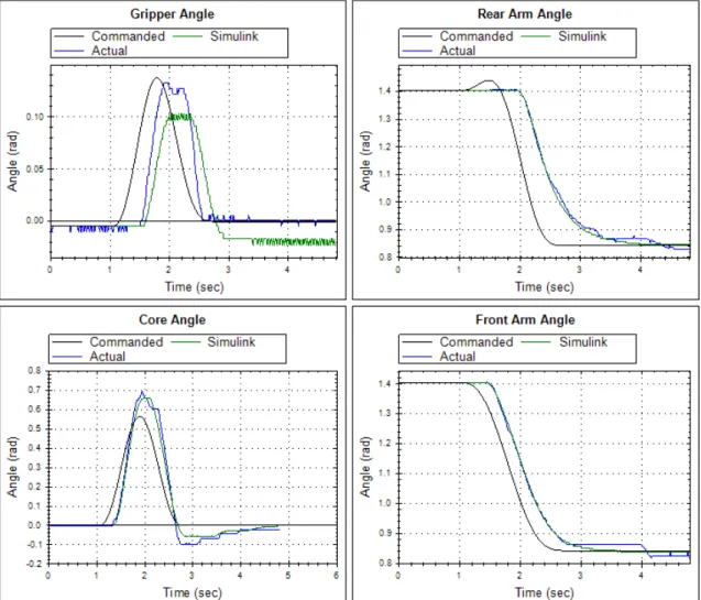
Since there is a delay between the trajectory command and the robot's movement (visible below in Figure 6.1), the final common trajectory position command was held steady at the end of each suspension clamp test for two seconds. An improvement to the PID controller would be to "turn off" the integrator when the robot has reached the desired set point with sufficient accuracy. The development of the Simulink model provided much insight into the behavior of the joint angle and current profiles seen in Figure 6.1 and Figure 6.8.
The ID model, Simulink model and actual current profiles for this test are shown in Figure 6.11. As in Figure 6.8, the Simulink model and the actual current profiles agree sufficiently to give confidence in the overall engineering solution.
Jumper manoeuvre
High Voltage Testing
Conclusion
Conclusion
Evaluation of Objectives and Specifications
The tests showed that the Simulink model of the robot was sufficiently detailed to predict the behavior of the robot. The techniques developed for trajectory interval time optimization based on the Simulink model were verified by the accuracy of the current profile predictions. It is clear from the work presented that the specifications outlined in the thesis allowed the required goals of the robot to be achieved.
It has been shown that the robot's charging needs can be minimized to extend the potential inspection time. Furthermore, the use of an autonomous obstacle avoidance scheme makes the operation of the robot simple and energy efficient by removing direct human control.
Improvements
The simulation results showed that the components of time splice B can be optimized to minimize such a cost function using the numerical simplex method. The predicted actuator cost function profiles using both models were consistent and had distinct minima around which the cost function was not overly sensitive to small variations in the input parameters. It has been demonstrated in experiments that the PLIR is capable of executing these optimized trajectories to successfully bypass the obstacle.
Finally, high voltage tests performed on the PLIR validated the robustness of the engineering design.
Concluding Remark
Optimizing Path Planning of Robotic Manipulators Considering System Dynamics”. Development and control of an autonomous robot for inspection of obstacles for high-voltage transmission lines. A new self-navigating inspection robot along a high-voltage transmission line and its application”. International Conference on Intelligent Robotics and Applications.
Control of an inspection robot for 110kV transmission lines based on expert system planning methods”.
Appendix A
PLIR Parameters
Simulink Model Parameters
PID Controller Parameters
Appendix B
Software
PLIR Trajectory Solver software
Simulink PLIR Model
Videos
Appendix C
Hardware
Ground Station Computer Specifications
On-board Computer Specifications