Inverse Air Entry Value or Bubbling Pressure (α) 58
Typically, α represents the inverse of the critical suction value at which the largest pores in the soil matrix begin to lose water (Rassam et al., 2003). As α is lowered in HYDRUS-2D, similar to clay soils, more matric suction is required for the soil to begin to drain the largest pores. As α increases in HYDRUS-2D, it behaves like a sandier soil that requires less matric suction from the soil to start draining larger pores, and this tendency holds until all available water is drained from the soil.
Pore Size Distribution Index (n) 58
Saturated Hydraulic Conductivity (Ks) 58
The simulations showed that the most sensitive parameters were the inverse of the air entrainment value or bubble pressure (α), the pore size distribution index (n) and the saturated hydraulic conductivity (Ks).
RESULTS AND DISCUSSION 60
East facing Hillslope and Wetland Transect
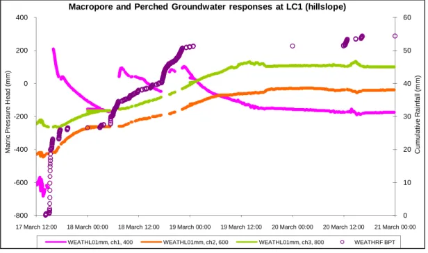
The simulated stress time series at this shallow depth showed close agreement with the observed data, with the summer stresses being accurate. The simulated values for this depth at LC 8 and LC 9 were reasonably modeled, but were mostly undersimulated with the general shape following that of the observed datum well. With the onset of the spring rains, the responses from each site at this depth vary.
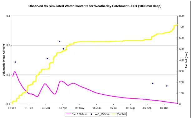
The deeper groundwater component (approximately 800 to 900 mm deep) represents slow unsaturated redistribution of groundwater to the bedrock with delivery of unsaturated water to the lower slopes as well as groundwater contributing to a marsh groundwater component in this transect, as summarized in Figures 3.8 and 3.9 respectively . This deeper groundwater component was adequately simulated based on visual comparison with the observed values. The simulated stresses for this deeper groundwater component were modeled well, with the simulated values being close to those of the observed data, but the peaks and troughs were out of phase.
The stresses at LC 10 responded favorably, but the responses occurred faster and paralleled the observed data, but were over-simulated. This deep groundwater component was simulated acceptably, based on visual comparison with the observed values. The simulated stresses for this deep groundwater component were well modeled, with the modeled values close to the observed data.
The winter recession is well modelled, with a stable decrease in stress noted close to the observed data.
Goodness of fit Statistics 83
The summer stress responded to larger precipitation events as can be seen in Figures D.22, D.27 and D.32 in Appendix D, but the responses were predictably delayed and sometimes the simulation responded too dramatically. The simulated stress time series and water content for Lower Catchment 8 (LC 8) to Lower Catchment 10 (LC 10) are included in Appendix D. The simulated stress was compared to the observed stress for each of the sites, at the same times, to ' to produce good statistics.
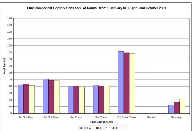
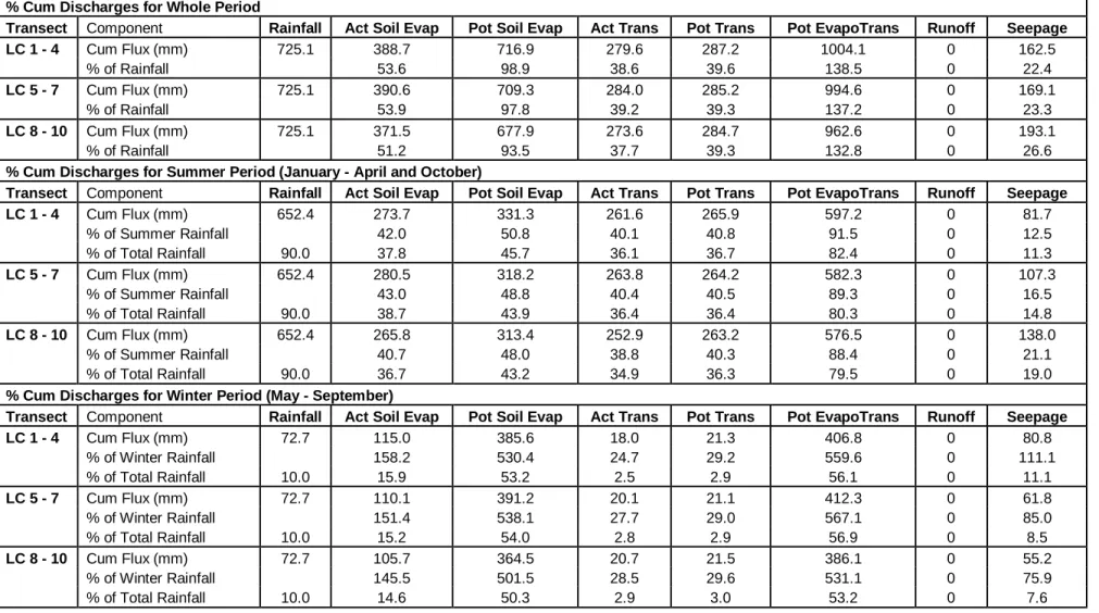
Cumulative Contributing Hillslopes Flux Results 84
- Cumulative fluxes for the West facing Upper
- Cumulative fluxes for the West facing Wetland
- Cumulative fluxes for the East facing
The simulation of the observed stresses for LC 5 at 740 mm depth was moderate, as shown in Figure D.7. The simulation of the observed stresses for LC 5 at a depth of 1280 mm was reasonable, with the simulated values remaining close to the observed data (Figure D.9). The simulation of the observed stresses and water contents for LC 7 at 460 mm depth was good, with the simulated values following the trends of the observed data well (Figure D.13).
The simulation of the observed stresses for LC 7 at 880 mm depth was satisfactory from visual analysis, with the simulated values continuing in close agreement with the observed data (Figure D.15). The simulation of the observed stresses for LC 7 at 1100 mm depth was excellent considering the depth, with the simulated values continuing to be close to the observed data (Figure D.17). The simulation of the observed stresses for LC 8 at 1450 mm depth was remarkable considering the depth, with the simulated values continuing to be proximal to.
The simulation of the observed stresses for LC 10 at 530 mm depth was good as can be seen in figure D.28. Simulation of the observed stresses for LC 10 at 830 mm depth was acceptable by visual comparison, with the simulated values continuing in the vicinity of. The simulation of the observed stresses for LC 10 at 1390 mm depth was adequate, especially considering the depth, with the simulated values remaining proximal to the observed data when compared visually (Figure D.32).
The simulated stress did not capably capture the complex relationships of the groundwater dynamics, but the values remained proximal to the observed data.
Seepage Hydrographs of the Contributing Hillslopes 94
- Seepage Hydrograph for the West facing Upper
- Seepage Hydrograph for the West facing Wetland
- Seepage Hydrograph for the East facing
SUMMARY AND CONCLUSIONS 97
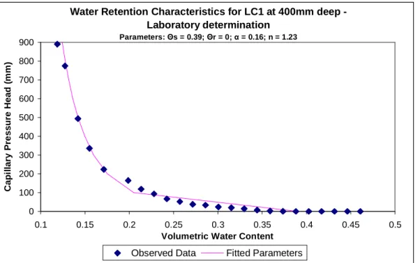
The use of transfer functions should offer a comprehensive quantification of the contributing hillslopes when assessing the contributions to the Weatherley catchment stream. From laboratory suction tests previously carried out on soils from the Weatherley catchment (Lorentz et al., 2001), water retention curves were plotted for the nest sites at different depths along the transects, which were then used to test different combinations of soil hydraulic properties. Rough estimates of the water retention properties are determined from observed data and then refined during modeling.
The timing of the stress response to precipitation events was generally well simulated, with the summer responses being fast and consistent. Cumulative fluxes were created where the various contributions of the components of the Weatherley catchment's soil dynamics are summarized in the form of high and low flow comparisons as well as comparisons of the components of each of the transects. The residence times of the uphill groundwater would also be longer with the stored groundwater only coming from the hillside as seepage during the winter period.
The seepage hydrograph for LC 1 – 4 shows both large, rapid responses and smaller responses to rainfall, depending on the preceding moisture conditions and the characteristics of the rainfall being responded to. The seepage hydrograph for LC 5 – 7 also shows large, rapid responses and smaller responses to rainfall, depending on the preceding moisture conditions and the characteristics of the rainfall being responded to. The responses of LC 8 – 10 do not appear to vary in magnitude or timing depending on the preceding moisture conditions and the characteristics of the rainfall responded to, as do the seepage responses of the other two transects.
This thesis aims to provide an understanding of the subsurface processes occurring in the Weatherley catchment, and subsequently describe and quantify the fluxes entering and leaving the contributing hillslopes.
RECOMMENDATIONS FOR FUTURE RESEARCH 103
The suggested transfer function model for the Weatherley catchment needs to be further reviewed and refined in relation to the various source zones such as macropore (preferential) flow, which contribute to the generation of streamflow. Extending the work done in this thesis to the rest of the Mooi River catchment, with more field studies in the larger catchment regarding land use, soil, land cover, geology, areas contributing to the flow of streams and a comprehensive time series study. Monitoring within the Weatherley catchment should continue, in light of recent afforestation, in relation to rainfall, streamflow, sediment yield, surface runoff, tensiometer, piezometer and well data, groundwater flows and subsurface flows.
The effective management of this pristine research basin is somewhat compromised by the lack of training and implementation of transparency in defining the various duties and tasks that flow from data capture to data entry into the Weatherley database. This type of flow in modeling is important because it contributes to rapid feedbacks within a catchment, which has implications for flood hydrology and sediment yield. A more detailed sampling study of the Weatherley watershed with natural isotopes or tracer chemical species should be undertaken.
A study of the near-stream flow generation mechanisms in the Weatherley catchment needs to be conducted to qualify and quantify the fluxes associated with plume flow and groundwater scouring phenomena during and after rainfall events. This study should also reveal information about the amounts and intensities of precipitation that initiate these types of flow-generating mechanisms at different antecedent moisture contents. The groundwater flow component will provide greater accuracy for all simulations, but especially for the wetland transect (LC 5 – 7), where a lot of fast and slow flow responses are generated by the fluctuating water table.
This thesis can then be used later in groundwater release studies regarding the cumulative effects of base flows from small watersheds to the large watershed scale and in studies of low discharge accumulation.
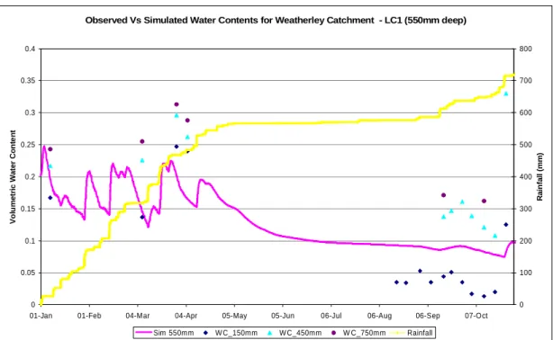
The simulated water content for LC 5 at 740 mm depth performed poorly compared to the observed data, showing little response in contrast to the opposite situation found in the observed data (Figure D.8). The simulated water content values were poorly simulated when visually compared to the observed data for LC 5 at 1280 mm deep, as can be seen from Figure D.10. The simulated water content for LC7 at 460 mm depth performed poorly compared to the observed data, as can be seen in Figure D.14.
The simulated water content values were poor visually compared to the observed data for LC 7 at 880 mm deep (Figure D.16). The simulation of the observed stresses and water content for LC 8 at 490 mm deep was a decent one from visual inspection, with the simulated values closely following the trends in the observed data. The simulated water content for LC8 at 490 mm depth performed poorly compared to the observed data from visual analysis (Figure D.19).
The simulation of the observed stresses for LC 8 at 820 mm depth was acceptable by visual assessment, with the simulated values remaining close to the observed data (Figure D.20), but the simulation tended to under-simulate throughout the period. The simulated water content values were of poor quality compared to the observed data for LC 8 at 820 mm deep (Figure D.21). The simulated water content values were ineffectively modeled when visually compared to the observed data for LC 8 at 1450 mm deep (Figure D.23).
The simulated water content for LC 10 at 530 mm deep performed well when visually compared to the observed data record, but was found to be inaccurate during spring precipitation, as can be seen in Figure D.29. The simulated water content values were adequate when visually compared to the observed data for LC 10 at 830 mm deep (Figure D.31). The simulated water content values were modeled tolerably when compared visually with the observed data for LC 10 at 1390 mm deep (Figure D.33).
APPENDICES 120