This is the first study of the errors of the Bakshi, Kapadia, and Madan (2003) risk-neutral moment estimators under the Duffie, Pan, and Singleton (2000) affine jump-diffusion model benchmarked against their true values. The BKM estimators have been used by many academics and practitioners to calculate risk-neutral moments; this method is also used to calculate the Chicago Board Options Exchange (CBOE) Skewness Index (SKEW)1, the forward indicator of tail risk or crash risk for the S&P 500 Index. Some papers have analyzed the errors of the BKM estimators, but they either do not have a clear/accurate benchmark or use oversimplified-unrealistic models.
The CBOE SKEW, the higher-order version of CBOE volatility index (VIX), was created based on the BKM risk-neutral skewness estimator following the success of the CBOE VIX. Vasquez (2017) studies the term structure of the implied volatility and finds that frontier portfolios with high slopes outperform those with low slopes both economically and statistically. Bakshi and Madan (2006) form a theoretical link between risk-neutral volatility and the higher-order moments of the physical volatility.
Under the Bates (1996) model, Ammann and Feser (2019) study the robustness of interpolating (cubic spline and kernel) and extrapolating (constant and linear) the implied volatility surface using a “plain-vanilla” implementation of BKM ( without any interpolation/extrapolation) as a benchmark. They find that interpolation and extrapolation help improve the information content of the estimator. In this paper, the errors of the BKM skewness estimator are analyzed using virtual options created using the Duffie, Pan, and Singleton (2000) (henceforth DPS) (double jump) affine jump diffusion model against closed-form exact skewness benchmarks which are derived from Zhang et al.
When a jump occurs, the marginal distribution of the jump size in variance y is exponential with mean µy.
Calibrating the Model
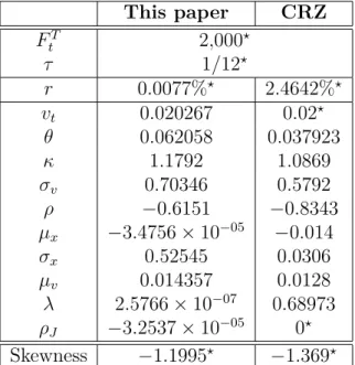
A common method is the two-step iterative procedure used by Christoffersen, Heston, and Jacobs (2009), Luo and Zhang (2012), Zhang et al. The two-step iterative procedure is generally to initialize the process by setting a set of initial values for the structural parameters and then (1) with the given set of structural parameters, optimize to find the latent variables and then (2) with the latent variables optimize to find the structural parameters. For clarity, since calibration is not the focus of this paper, equal weight is assigned.
Finally, with all structural variables fixed, the latent variable, the current variance vt, is calibrated for each day using the VIX. The iterative two-step calibration method is potentially faster as fewer parameters need to be calibrated simultaneously, but depending on how the parameters are separated between steps (1) and (2), there may be some fluctuations that can slow down convergence.
Generate Virtual Option Prices
The term to maturity is set at one month because they are usually the most liquid.
Deriving the Exact Skewness
The range can be decomposed into four components: T CMH, V ARH, T CMJ and V ARJ corresponding to the third central moment (T CM) and variance (V AR) contribution of Heston (1993) (H) and jumps ( J) , respectively. An alternative way to derive bias is to use moment generating functions or cumulant generating functions, similar to how CRZ derived their estimators.7 As mentioned in CRZ, the method of Zhang et al. The solution presented in equation (B.6) is verified using cumulant generating functions derived from equation (6) (which is the same method as CRZ, but without the finite difference derivatives).
Interpolation/Extrapolation
A key parameter for kernel regressions is the bandwidth, which can be found using the Nadaraya-Watson kernel regression estimator (Nadaraya (1964) and Watson (1964)) and optimized based on its mean squared error with leave-one-out cross-validation.
4 Data
5 Results
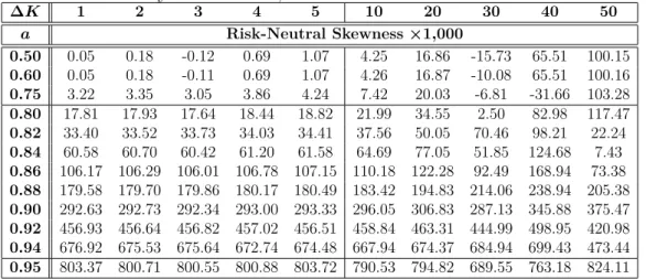
This discrepancy in step size is most likely due to the oscillatory nature of its relationship with error. Option strikes are denser near the money and out-of-the-money strikes tend to be rarer. Although a step size of $4 would be sufficient to obtain an error of less than 10−3 if the limit control factor is 0.60 - over the entire domain, the step size must all be $4.
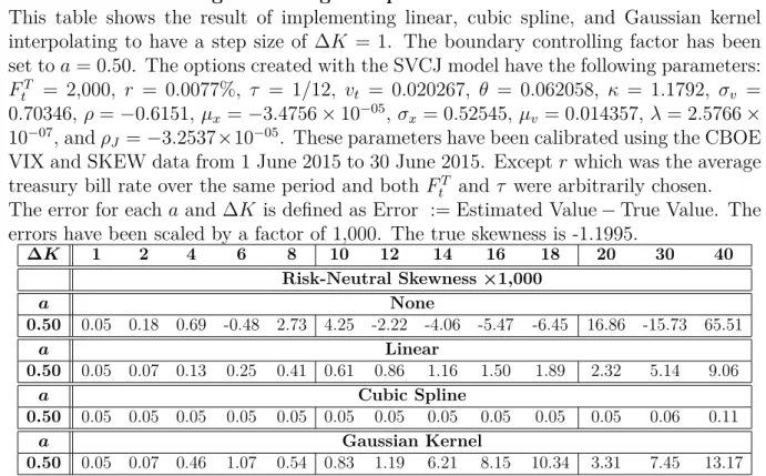
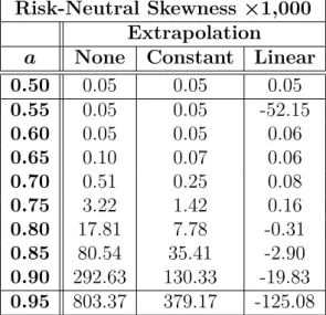
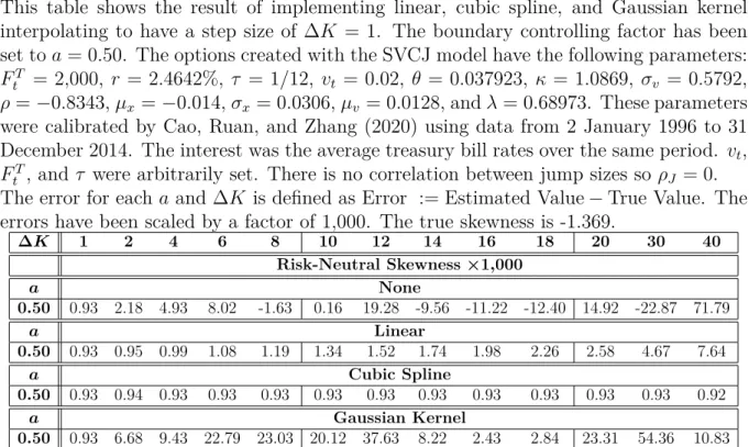
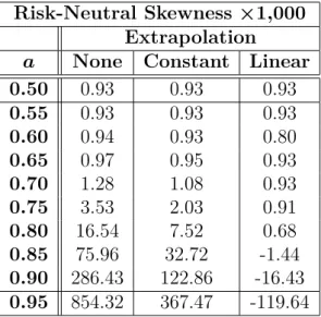
These interpolation methods are used when the limit control factor is 0.50 and interpolation is performed to achieve a step size of $1. Pruning is generally a larger source of error, so extrapolation techniques must be used. Both extrapolation methods generally reduce errors, with the linear extrapolation approach producing smaller errors, especially when the boundary control factor is large.
The parameters for Tables V to VII were calibrated by CRZ using data from January 2, 1996 to December 31, 2014. In general, past market conditions show that the direct application of the BKM risk-neutral skewness estimator to obtain SKEW without interpolation and extrapolation is unlikely to be accurate. Applying a combination of cubic spline interpolation to $1 and constant interpolation to have strike prices from half the forward price to double the forward price (a bounding factor of 0.50) should consistently reduce errors to less than 10- 3 to be.
6 Conclusion
Chang, Bo Young, Peter Christoffersen and Kris Jacobs, 2013, Market Asymmetry Risk and the Cross Section of Stock Returns, Journal of Financial Economics. Chatrath, Arjun, Hong Miao, Sanjay Ramchander, and Tianyang Wang, 2016, An overview of crude oil flow characteristics: Evidence from non-risk-neutral moments, Energy Economics. Chordia, Tarun, Tse-Chun Lin and Vincent Xiang, 2020, Risk-neutral skewness, informed trading, and the cross section of stock returns, Journal of Financial and Quantitative Analysis, 1-25.
Christoffersen, Peter, Steven Heston and Kris Jacobs, 2009, The shape and term structure of the index option smirk: why multifactor stochastic volatility models work so well, Management Science. Dittmar and Allaudeen Hameed, 2020, Implied default probability and loss given default from option pricing, Journal of Financial Econometrics. Dennis, Patrick and Stewart Mayhew, 2002, Risk neutral bias: evidence from stock options, Journal of Financial and Quantitative Analysis.
Duffie, Darrell, Jun Pan and Kenneth Singleton, 2000, Transform analysis and asset pricing for affine jump diffusions, Econometrica. Heston, Steven L., 1993, A closed-form solution for stochastic volatility options with applications to bond and currency options, Review of Financial Studies. Hollstein, Fabian, Marcel Prokopczuk, and Chardin Wese Simen, 2020, The contingent pricing model for capital assets revisited: evidence from high-frequency betas, Management Science.
Huang, Jing-zhi and Liuren Wu, 2004, Specification analysis of option pricing models based on time-varying Lévy processes, Journal of Finance. Lee, Geul and Li Yang, 2015, Effect of Truncation on Model-Free Implicit Moment Estimator, Available at SSRN: https://ssrn.com/abstract=2485513. Liu, Zhangxin, and Thijs van der Heijden, 2016, Moments and Risk-Neutral Proxies, available at SSRN: https://ssrn.com/abstract=2641559.
Neumann, Michael and George Skiadopoulos, 2013, Anticipatory Dynamics in Higher-Order Risk-Neutral Moments: Evidence from S&P 500 Options, Journal of Financial and Quantitative Analysis. Stilger, Przemysław S., Alexandros Kostakis and Ser-Huang Poon, 2017, What risk-neutral asymmetry tells us about future stock returns. Vasquez, Aurelio, 2017, Term structures of equity volatility and the cross section of option returns, Journal of Financial and Quantitative Analysis.
Appendix
A BKM Derivation
B Exact Skewness
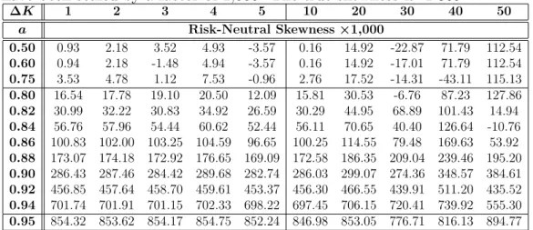
Finally, by adding the correlated jumps in volatility to obtain the DPS model (Equation (5)), we can find that the asymmetry. This table shows the error of the BKM asymmetry estimator for different boundary control factors, a, and step sizes, ∆K. These parameters were calibrated using CBOE VIX and SKEW data from June 1, 2015 to June 30, 2015.
Except that r was the average government bond yield over the same period and both FtT and τ were chosen randomly. This table shows the result of implementing linear, cubic spline and Gaussian kernel interpolation to get a step size of ∆K = 1. Except, this was the average government bond yield over the same period and both FtT and τ were chosen randomly.
This table shows the result of implementing constant and linear extrapolation to have a boundary control factor of a = 0.50.