On the balance sheet, this approximation is presented through three accounts: (1) total assets (Asset), (2) gross plant, property and equipment (GPPE) and (3) net plant, property and equipment (NPPE). On the one hand, it is reflected in the firm's position in the supply chain.
METHODS
Phase 1: Data Collection
We exclude these estimates from the data set and end up with a highly unbalanced panel of 12,811 firm fiscal year observations (2,316 firms globally over 11 fiscal years). 12 Income is identified as the key feature in our forecasting models, so all model calibration includes income as one of the regressors.
Phase 3: K-Fold Division
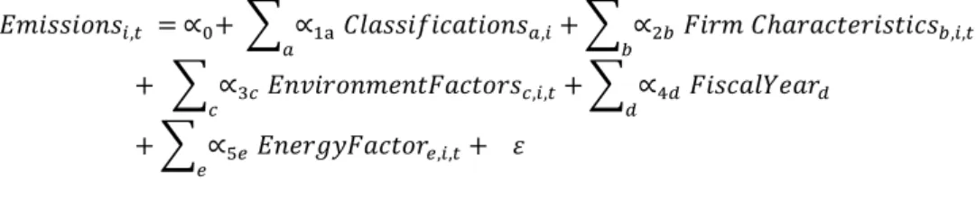
𝐸𝑛𝑣𝑖𝑟𝑜𝑛𝑚𝑒𝑛𝑡𝐹𝑎𝑐𝑡𝑜𝑟𝑠𝑐,𝑖,𝑡 is a vector of dummy variables c representing the carbon laws and national income group of firm i. 𝐹𝑢𝑒𝑙𝐼𝑛𝑡𝑒𝑛𝑖,𝑡 is the carbon intensity of the national mix of the country with the headquarters of company i at time t.
Phase 5: Building Base Learners
The hidden units ℎ𝑘(𝑥) are then used to predict the target variable as illustrated in equation (12), where 𝛾𝑘 is the effect of the kth hidden unit on the target variable y. Here 𝑤𝑗𝑘 is the effect of the predictor 𝑥𝑗 on the hidden unit ℎ𝑘(𝑥) (see Equation (11a)), 𝛾𝑘 is the effect of the hidden unit ℎ𝑘(𝑥1) (see Equ variable) (see Equation (11a)).
Phase 6: Building Meta Learners
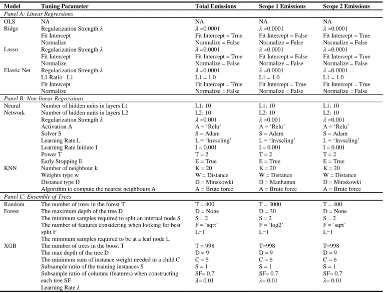
Neural Network Number of hidden units in layers L1 Number of hidden units in layers L2 Regularization strength 𝜆 Activation A. Random forest The number of trees in the forest T The maximum depth of the tree D. Subsample ratio of the training cases S Subsample ratio of columns (features) when each tree be built C.
The implementation of stacked generalization is the two-level procedures: the first step is to generate the first-level prediction output using a variety of first-level base learners; the second step is to generate second-level prediction on first-level predictions using a second-level algorithm (meta-learner). For each kth fold, the base learner 𝐵𝑗 is trained on the observations from k-1 remaining folds, and a prediction vector 𝑜𝑗𝑘 of n/k size is generated for this fold. The process is then continued with all other base learners to form the matrix of J vectors of secondary predictors O= {𝑜1, 𝑜2, .
To generalize stacking, we use three sophisticated algorithms to combine the predictions of the 8 basic learners in phase 5, namely OLS, ElasticNet, and XGB. Similar to the base learners, we also perform hyperparameter optimization to improve the prediction accuracy of the metalearners. We also use the Sequence Grid Search strategy to achieve the best hyperparameter settings, and the search space follows the hyperparameter setting of the basic learners (as shown in Table 4).
Phase 7: Model Evaluation
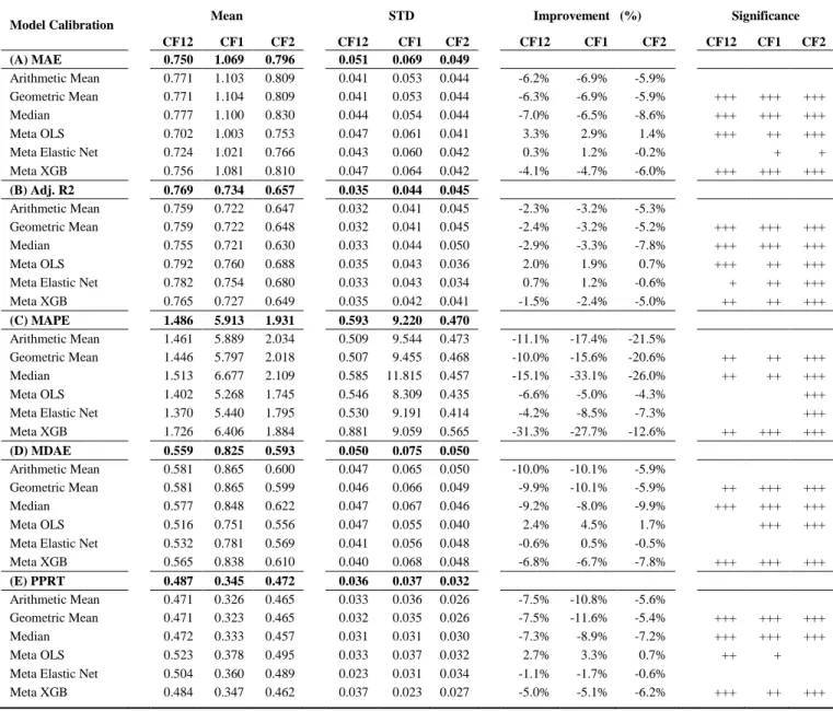
This process is performed exclusively on the validation dataset, and the estimation procedure follows Figure 2. The log-transformed MAE is quite straightforward to interpret, for example, if the MAE of log-transformed emissions is 0.5, it means that the MAE of untransformed emissions is equal to ( 𝑒0.5 − 1) or ~ 64.8% of the average emissions (e = 2.71828). To ensure that we adequately capture the degree of model performance, we also employ four supplementary metrics, namely Median Absolute Error (MDAE), Adjusted R2 (Adj. R2), Mean Absolute Percentage Error (MAPE), and Percentage of Prediction in Acceptance Range (IAR).
We include the adjusted R2 corresponding to the predictions of the log-transformed data as a measure of the explanatory power of the model. A limitation of adjusted R2 is that it assumes linearity between predictors and target variables. Following Griffin, Lont, and Sun (2017), we conduct further robustness tests to validate the predictive ability of the model.
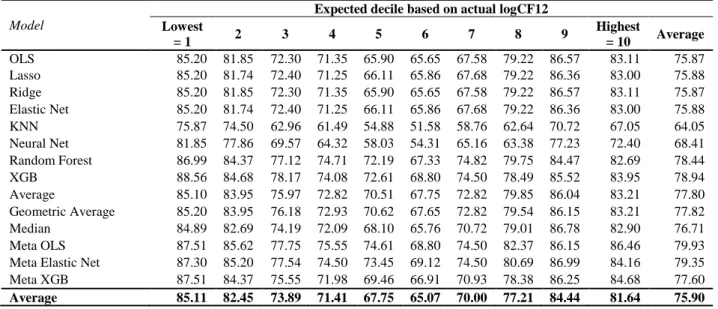
The first is Test of Decile Ranking, where we assign log-transformed emissions to deciles and calculate the percentage of predicted values that remain in the same or adjacent deciles with their actual data. The second is the Test of Mean Difference, where we perform a two-sided test to ensure that the average predicted value and the actual values are not statistically different over the years. Finally, we conduct Test of Bias, examining model performance for each reporting year and sector.
RESULTS
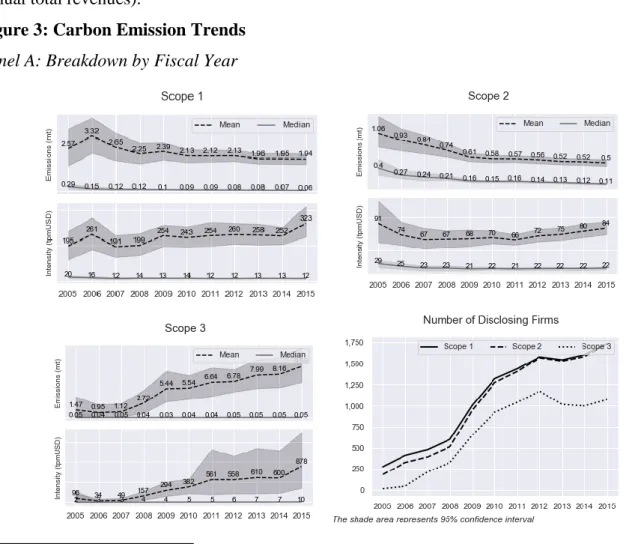
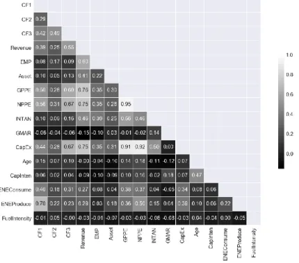
There is wide variation in carbon emissions across sectors, signaling a strong predictive power of industry classification. Meanwhile, if the company's home country has implemented carbon pricing on a nationwide coverage, the average carbon emission/intensity is lower in both Scope 1 and Scope 2. We use Pearson correlation as a baseline to measure the linear relationship between variables with normality distributions.
24 The Spearman value calculates the Pearson correlation between the rank values of two data and makes no assumptions about data distribution. We also perform a Pearson correlation analysis on log-transformed variables, which gives very similar results to Spearman rank. A closer look at the ratio values, namely asset age (Age) and capital intensity (CapInten) confirms our explanation, as companies with newer physical assets and less capital intensive are associated with a lower level of carbon emissions.
Interestingly enough, we hypothesize that energy consumption (EneConsume) is more closely related to Scope 2 (Pearson: 0.18, Spearman: 0.75), however, we find that its predictive power is even stronger in Scope 1 than Scope 2 (Pearson: 0.40, Spearman: 0.88). Last but not least, we find that national fuel mix helps explain CF2 to some extent (Pearson: 0.05, Spearman: 0.18). We observe strong co-movements between scale factors (for example, Pearson values between income and employees, assets, GPPE, NPPE, INTAN are, respectively, and 0.46), as well as between scale indicators and other predictors (for example, the Pearson correlation between Revenue and CapEx is 0.67).
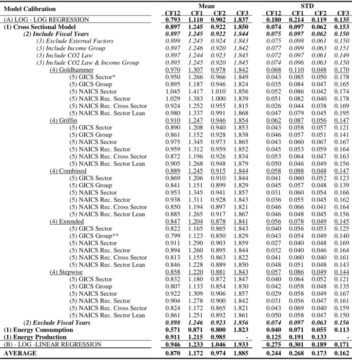
All figures are given using the mean and standard deviation of efficiency from 10-fold validation. The average PPAR of 41.3% suggests that nearly half of the observations are within the acceptable range. If a home country's ESG awareness affects a company's level of energy consumption, enacted legislation is more important than status (take the US as an example).
This strategy results in slightly degraded performance (increase the MAE by 0.04 for total emissions), but is still necessary to retain 25% of the data sets. For example, the optimal setting for Scope 1 comes from a similar model calibration to that of Total Emissions, but the Income Group factors are excluded from the list of predictors. For Scope 3, the step-by-step process excludes insignificant industrial groups from the forecast formula, but the Energy Group, the start of the carbon supply chain, has the highest.
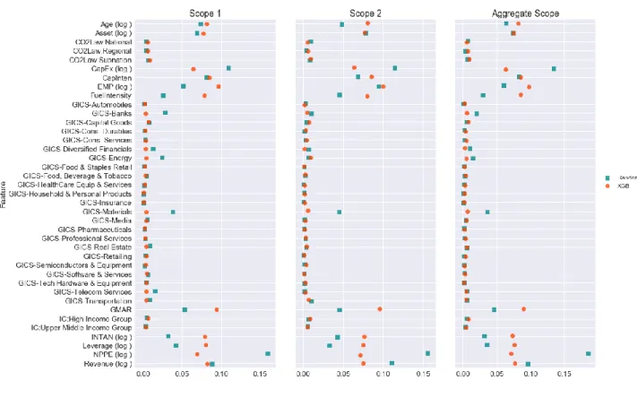
Notes They indicate that the prediction performance of the corresponding algorithm is better than the OLS model at 1%, 5% and 10% significance level. The problem of multicollinearity does not appear to be strong enough to degrade the performance of the OLS model, even when we choose to use an extended list of operation ranges and consider the same aspect with different approximations. For ensemble models, predictor importance is defined as a function of squared error reduction: “the improvement in squared error due to each predictor is summed within each tree in the ensemble (ie, each predictor gets a . improvement value for each tree)” (Kuhn & Johnson, 2013).
Meta Learner Performance
In general, the predictor significance profile in XGB has a steeper slope than XGB, this is because the trees in this case grow dependently (correlated structure). A similar pattern is found in Scope 1 and Scope 2 in isolation, with a greater emphasis on Employees for subsequent outreach.
Additional Robustness Test
Panel B shows the two-tailed test in which we perform a comparison between averages of forecast and actual emissions over years. The p-values in none of the years are significant, indicating that the average estimated log emissions and the actual log emissions do not differ significantly. In the current setting, we are aggregating all data points into one panel, regardless of fiscal years or industry classification.
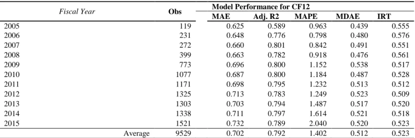
In terms of years, we observe a slightly higher predictive power in the first years of detection and 2007), probably due to the small sample size and lower variation. In terms of industry, we see the most accurate performance coming from Pharmaceuticals, Retail, Software &. 57 because the GICS Classification has no way of distinguishing between fossil fuel utility firms and green utility firms.
Our meta-learner algorithm shows superior performance in predicting emissions from SP 500 companies, with an average R2 of up to 82.8% for total emissions (see Table 12).
CONCLUSION
Investors' Business Daily Available at https://www.investors.com/politics/commentary/note-to-environmentalists-not-all-fossil-funers-are-the-same/. Forecasting CO2 emissions using an artificial neural network: the example of the sugar industry. Working Group on Climate-Related Financial Disclosures. Available at https://www.fsb-tcfd.org/publications/final-.
Available at https://financial.thomsonreuters.com/content/dam/openweb/documents/pdf/financial/esg-carbon-data-estimation-models.pdf. Prediction and Analysis of CO2 Emission in Chongqing for the Protection of the Environment and Public Health.
APPENDIX
Table 1 - NAICS Sector Reclassification
NAICSGroup TR Eikon 2012 NAICS Industry Group -4 city codes (312 industry groups) NAICSInd TR Eikon 2012 NAICS National Industry Classification - 6 city codes (1065 industries) GICSSector classification TR Eikon 1 for each of the 11 GICS industry sectors (11th is in interception) Classification. CF1 Asset4 Carbon footprints (GHGE emissions in scope 1) per company per reporting year CO2e tonnes. CF2 Asset4 Carbon footprints (GHGE emissions in scope 2) per company per reporting year CO2e ton.
CF3 Asset4 Carbon footprint (GHGE emissions in Field 3) per firm for the reporting year CO2e tonnes. CF12 Self-calculated carbon footprints (scope 1 and 2 GHGE emissions) per firm for reporting year CO2e ton CI1 Self-calculated carbon intensity (scope 3 GHGE emissions) per firm for reporting year CO2e ton /$ USM CI2 Self-calculated carbon intensity (GHGE emissions in field 1 and 2) per firm for the reporting year CO2e tonnes. USM CI3 Self-calculated carbon intensity (GHGE emissions in field 1 and 2) per firm for the reporting year CO2e tonnes.
USM CI12 Self-calculated carbon footprints (Scope 1 and 2 GHGE emissions) per company per reporting year per ton of CO2e. GPPE TR Eikon Gross tangible fixed assets per company at the end of the reporting year USD thousands. NPPE TR Eikon Net tangible fixed assets per company at the end of the reporting year in thousands of US dollars.
Age Self-calculated Gross fixed assets for depreciation costs per company at the end of the reporting year. CapInten Self-calculated gross tangible fixed assets per company divided by turnover at the end of the reporting year % Leverage Self-calculated Long-term debt divided by total assets at the end of the reporting year.